Survival Analysis in R

Author

David M. Miller, Sophia Z. Shalhout

Published

April 13, 2020

Abstract

In this post we provide a user guide on how to analyze Survival Data in R

Key points

This post provides a resource for navigating and applying the Survival Tools available in R.
- We provide an overview of time-to-event Survival Analysis in Clinical and Translational Research (CT Research).
- We outline the steps to creating Kaplan-Meier Curves and visualizing Hazard Ratios with Forest Plots and provide pearls on how to effectively analyze and plot data sets intended for Survival Analysis.
- We briefly describe the statistics behind Survival Analysis. Readers are referred to an abundance of resources available that provide a deeper explanation of the principles behind the statistical tests, which is beyond the scope of this post.
Skill Level: Intermediate
- Assumptions made by this post is that readers have some familiarity with basic biostatistics and R.
- Additional resources on various elements of Survival Analysis include: Fox and Weisberg, and Rickert

Background on Survival Analysis

Survival Analysis is one the most common types of time-to-event data analysis in medical research
Common objectives in Survival Analysis are:
1. Comparing the survival distribution between groups
2. Estimating the survival distribution
3. Modeling the effect of explanatory variables on the outcome variable
In Clinical and Translational Research (CT Research) there are numerous applications for time-to-event analyses and various tools to conduct the above common objectives
- For example, in clinical trials, the two main analytic tasks in time-to-event evaluation are to:
  1. Test the equality of the treatment groups
  2. Estimate the magnitude of the treatment effect
- In CT Research the estimate of the magnitude of the treatment effect is often evaluated in the context of the estimation of risk of that treatment
  - For example, in order for a labeled claim to be approved by the U.S. Food and Drug Administration, the sponsor of a Investigational New Drug must establish that the proposed agent demonstrates a “positive risk-benefit assessment”
As Hajim Uno et al. describe it, when these two tasks are combined, one can use a “test/estimation” approach to evaluating time-to-event data
- Of note, there are different approaches to perform “test/estimation” analyses, though the combination of the log-rank test with the estimation of a Harzard Ratio is by far the most popular in medical research
  - Therefore, in this post, we will focus on how to perform these two tests on time-to-event data in R

Handling Dates

Time-to-event data is more complex than traditional continuous outcomes because two or three pieces of information are involved
In the simple case of a time-to-event when every subject starts at the same point (i.e. the beginning of a clinical trial), the two pieces of information are the time-to-event and an indicator of whether the event is a failure time or a censoring time
Often, survival data start as calendar dates rather than as survival times, and then we must convert dates into a usable form for R before we can complete any analysis.
If you are going to use Dates, they should be in YYYY-Month-Day format
- The as.Date() function can be applied to convert numbers in various charactor strings (e.g. “02/27/92”) into recognizable date formats
  - as.Date("02/27/92", "%m/%d/%y")
Often though, you will be using a discete time interval in days

Load Packages and Data Sets

Load the `survival` package

You need the survival package (which was created by Terry Therneau at Mayo)

library(devtools)
install_github('therneau/survival',dependencies=TRUE)
library(survival)

Load Other Packages

library(tidyverse)
library(knitr)
library(survminer)
library(survival)

Load Data Sets

Overview

We will use two main data sets for this tutorial which are built-in datasets:
- the veteran Data Set
- the colon Data Set
Let’s start by viewing the veteran data set

veteran <- veteran
kable(head(veteran))

trt	celltype	time	status	karno	diagtime	age	prior
1	squamous	72	1	60	7	69	0
1	squamous	411	1	70	5	64	10
1	squamous	228	1	60	3	38	0
1	squamous	126	1	60	9	63	10
1	squamous	118	1	70	11	65	10
1	squamous	10	1	20	5	49	0

Definition of Variables in Veteran Data Set
trt: 1=standard, 2=test
celltype: 1=squamous, 2=smallcell, 3=adeno, 4=large
time: survival time
status: censoring status
karno: Karnofsky performance score (100 = Normal; 0 = Dead)
diagtime: months from diagnosis to randomisation
age: in years
prior: prior therapy 0=no, 10=yes

Kaplan-Meier Estimator

Overview

The Kaplan-Meier curve is a nonparametric estimator of the survival distribution (i.e. the “estimation” component of the “test/estimation” approach to analysis of time-to-event data)
In their June 1958 paper in the Journal of the American Statistical Association, E.L. Kaplan and Paul Meier proposed a way to nonparametrically estimate S(t), even in the presence of censoring

Analyze Survival Data in R

`Surv()` Function

The Surv() function takes the following arguments:

function (time, time2, event, type = c(“right”, “left”, “interval”, “counting”, “interval2”, “mstate”), origin = 0)

To use the functions in the survival library, we will have to specify both the “survival time” and the “failure indicator” in the Surv() function
When we use the Surv() function, we specify the time variable first and the failure indicator second
In R, the failure indicator should equal 1 for subjects with the event and equal 0 for subjects who are right censored
You can type time = and event = as we will see below

Build Surv Object

# Generate Surv Object
veteran_Surv <- Surv(time = veteran$time, event = veteran$status)

In the above, the variable “time” is the time variable and “status” connotes whether or not a subject had the event (“status = 1”) or was right censored (“status = 0”)

# View Surv Object
head(veteran_Surv, 50)

 [1]  72  411  228  126  118   10   82  110  314  100+  42    8  144   25+  11 
[16]  30  384    4   54   13  123+  97+ 153   59  117   16  151   22   56   21 
[31]  18  139   20   31   52  287   18   51  122   27   54    7   63  392   10 
[46]   8   92   35  117  132

In the list above, each time that has a “+” connotes that it was censored in the analysis

Analyze the Survival Data with the `survfit()` function

To analyze the data we use the survfit() function, in which you will place the Surv Object of interest (here veteran_Surv) followed by a “~” and a predictor.
- If you want a single curve, with no specific predictor, use “1”.
- If there is a predictor variable for which you want to compare the outcome of, you will place that variable to the right of the “~”.
Then place the data you want evaluated to the right of the “,”, as below.

Generate a KM Curve

Overview

First let’s generate a KM Curve wiht No Predictor
We will then show how to plot that basic curve
Then we will demontrate how to generate a KM Curve stratifed by a Explanatory Variable (aka a “Predictor”)

# Generate Survfit Object
veteran_Survfit <- survfit(veteran_Surv ~ 1, data = veteran)

# View Survfit Analysis at various time points
summary(veteran_Survfit, times = c(1, 50, 100*(1:10)))

Call: survfit(formula = veteran_Surv ~ 1, data = veteran)

 time n.risk n.event survival std.err lower 95% CI upper 95% CI
    1    137       2    0.985  0.0102      0.96552       1.0000
   50     84      50    0.619  0.0416      0.54299       0.7064
  100     55      27    0.418  0.0425      0.34251       0.5101
  200     25      26    0.205  0.0360      0.14560       0.2895
  300     13      10    0.117  0.0295      0.07147       0.1917
  400      6       7    0.054  0.0211      0.02509       0.1163
  500      4       2    0.036  0.0175      0.01389       0.0934
  600      2       2    0.018  0.0126      0.00459       0.0707
  700      2       0    0.018  0.0126      0.00459       0.0707
  800      2       0    0.018  0.0126      0.00459       0.0707
  900      2       0    0.018  0.0126      0.00459       0.0707

The “times” argument in the “summary()” function allows you to control which time intervals you print
If you want to view the output of the analysis of the total output, use the following call
Of note, you could have also used the following code to generate the same survfit object veteran_Survfit <- survfit(Surv(time = veteran$time, event = veteran$status) ~ 1, data = veteran)

veteran_Survfit

Call: survfit(formula = veteran_Surv ~ 1, data = veteran)

       n events median 0.95LCL 0.95UCL
[1,] 137    128     80      52     105

You can also view the median of the data with the following code

median(veteran$time)

[1] 80

Visualizing Survival Data

Overview

You can plot your survival data with base R or other functions such as ggsurvplot()

Plot Data Using Base `R`

The plot() function can be used to take a surv object and generate a basic Kaplan-Meier curve, as below

plot(veteran_Surv, 
     main = "Overall Survival", #plot title
     sub = "Unstratified Cohort", # Subtitle
     xlab="Days", 
     ylab="Survival Probability" )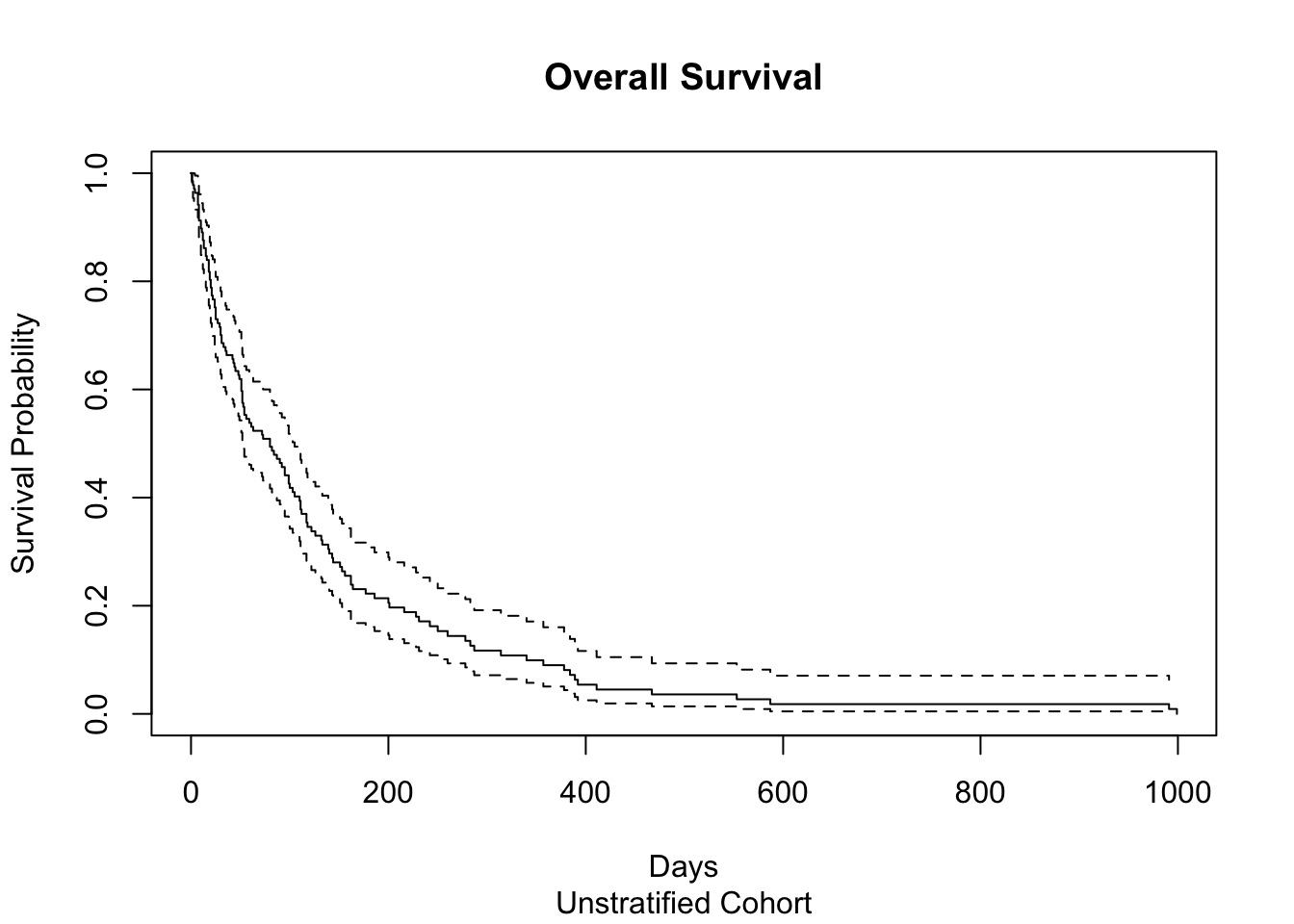

Plot Data Using `ggsurvplot`

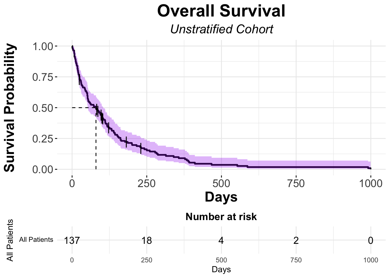
The ggsurvplot can generate visually appealing plots

# Kaplan-Meier using ggsurvplot
ggsurvplot(fit = veteran_Survfit, 
           data = veteran,
           ####### Format Title #######
           title = "Overall Survival",
           subtitle = "Unstratified Cohort",
           font.title = c(22, "bold", "black"),
           ggtheme = theme_minimal() + theme(plot.title = element_text(hjust = 0.5, face = "bold"))+
             theme(plot.subtitle = element_text(hjust = 0.5, size = 16, face = "italic")), # center and bold title and subtitle
           ####### Format Axes #######
           xlab="Days", # changes xlabel,
           ylab = "Survival Probability",
           font.x=c(18,"bold"), # changes x axis labels
           font.y=c(18,"bold"), # changes y axis labels
           font.xtickslab=c(14,"plain"), # changes the tick label on x axis
           font.ytickslab=c(14,"plain"),
           ####### Format Curve Lines #######
           color = "black",
           ####### Censor Details ########
           censor.shape="|",
           censor.size = 5,
           ####### Confidence Intervals ########
           conf.int = TRUE, # To Remove conf intervals use "FALSE"
           conf.int.fill = "purple", # fill color to be used for confidence interval
           surv.median.line = "hv", # allowed values include one of c("none", "hv", "h", "v"). v: vertical, h:horizontal
           ######## Format Legend #######
           legend.title = "All Patients",
           legend.labs = "All Patients", # Change the Strata Legend
           ######## Risk Table #######
           risk.table = TRUE, # Adds Risk Table
           risk.table.height = 0.25, # Adjusts the height of the risk table (default is 0.25)
           risk.table.fontsize = 4.5
           )

KM Curves with a Predictor

Overview

This is typically a more common use of the KM method, where one wants to test a hypothesis that a drug prolongs Overall Survival, for example

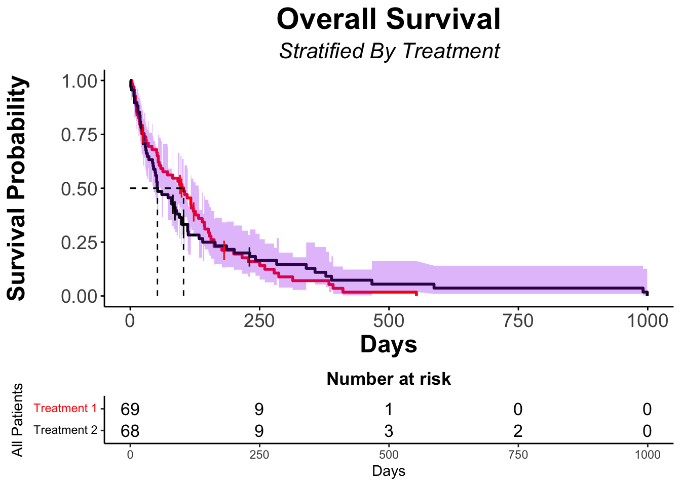
Stratify Analysis Based on Treatment (Standard vs. Experimental)

# Generate Survfit_trt Object
veteran_Survfit_trt <- survfit(veteran_Surv ~ veteran$trt, data = veteran)

# View Survfit Analysis at various time points
summary(veteran_Survfit_trt, times = c(1, 50, 100*(1:10)))

Call: survfit(formula = veteran_Surv ~ veteran$trt, data = veteran)

                veteran$trt=1 
 time n.risk n.event survival std.err lower 95% CI upper 95% CI
    1     69       0   1.0000  0.0000      1.00000        1.000
   50     46      22   0.6797  0.0563      0.57782        0.800
  100     34      12   0.5020  0.0606      0.39615        0.636
  200     12      19   0.1947  0.0501      0.11761        0.322
  300      5       6   0.0885  0.0371      0.03896        0.201
  400      2       3   0.0354  0.0244      0.00917        0.137
  500      1       1   0.0177  0.0175      0.00256        0.123

                veteran$trt=2 
 time n.risk n.event survival std.err lower 95% CI upper 95% CI
    1     68       2   0.9706  0.0205      0.93125        1.000
   50     38      28   0.5588  0.0602      0.45244        0.690
  100     21      15   0.3326  0.0578      0.23670        0.467
  200     13       7   0.2162  0.0517      0.13538        0.345
  300      8       4   0.1464  0.0454      0.07973        0.269
  400      4       4   0.0732  0.0344      0.02912        0.184
  500      3       1   0.0549  0.0303      0.01861        0.162
  600      2       1   0.0366  0.0251      0.00953        0.140
  700      2       0   0.0366  0.0251      0.00953        0.140
  800      2       0   0.0366  0.0251      0.00953        0.140
  900      2       0   0.0366  0.0251      0.00953        0.140

veteran_Survfit_trt

Call: survfit(formula = veteran_Surv ~ veteran$trt, data = veteran)

               n events median 0.95LCL 0.95UCL
veteran$trt=1 69     64  103.0      59     132
veteran$trt=2 68     64   52.5      44      95

# Kaplan-Meier using ggsurvplot
ggsurvplot(fit = veteran_Survfit_trt, 
           data = veteran,
           ####### Format Title #######
           title = "Overall Survival",
           subtitle = "Stratified By Treatment",
           font.title = c(22, "bold", "black"),
           ggtheme = theme_classic() + theme(plot.title = element_text(hjust = 0.5, face = "bold"))+ # theme_classic will give a white background with no lines on the plot
             theme(plot.subtitle = element_text(hjust = 0.5, size = 16, face = "italic")), 
           ####### Format Axes #######
           xlab="Days", # changes xlabel,
           ylab = "Survival Probability",
           font.x=c(18,"bold"), # changes x axis labels
           font.y=c(18,"bold"), # changes y axis labels
           font.xtickslab=c(14,"plain"), # changes the tick label on x axis
           font.ytickslab=c(14,"plain"),
           ####### Format Curve Lines #######
           palette = c("red","black"),
           ####### Censor Details ########
           censor = TRUE, # logical value. If TRUE, censors will be drawn,
           censor.shape="|",
           censor.size = 5,
           ####### Confidence Intervals ########
           conf.int = TRUE, # To Remove conf intervals use "FALSE"
           conf.int.fill = "purple", # fill color to be used for confidence interval
           surv.median.line = "hv", # allowed values include one of c("none", "hv", "h", "v"). v: vertical, h:horizontal
           ######## Format Legend #######
           legend = "none", # If you'd prefer more space for your plot, consider removing the legend
           legend.title = "All Patients",
           legend.labs = c("Treatment 1","Treatment 2"), # Change the Strata Legend
           ######## Risk Table #######
           risk.table = TRUE, # Adds Risk Table
           risk.table.height = 0.25 # Adjusts the height of the risk table (default is 0.25)
           )

Another Example of a KM stratified by an Explanatory Variable - Cell Type

# Generate Survfit_histo Object
veteran_Survfit_histo <- survfit(veteran_Surv ~ veteran$celltype, data = veteran)

# View Survfit Analysis at various time points
summary(veteran_Survfit_histo, times = c(1, 50, 100*(1:10)))

Call: survfit(formula = veteran_Surv ~ veteran$celltype, data = veteran)

                veteran$celltype=squamous 
 time n.risk n.event survival std.err lower 95% CI upper 95% CI
    1     35       2    0.943  0.0392       0.8690        1.000
   50     23       9    0.681  0.0794       0.5423        0.856
  100     20       2    0.622  0.0828       0.4793        0.808
  200     13       6    0.426  0.0873       0.2849        0.636
  300      8       4    0.288  0.0820       0.1650        0.503
  400      5       3    0.180  0.0711       0.0831        0.391
  500      3       2    0.108  0.0581       0.0377        0.310
  600      2       1    0.072  0.0487       0.0192        0.271
  700      2       0    0.072  0.0487       0.0192        0.271
  800      2       0    0.072  0.0487       0.0192        0.271
  900      2       0    0.072  0.0487       0.0192        0.271

                veteran$celltype=smallcell 
 time n.risk n.event survival std.err lower 95% CI upper 95% CI
    1     48       0   1.0000  0.0000       1.0000        1.000
   50     25      23   0.5208  0.0721       0.3971        0.683
  100     10      14   0.2257  0.0609       0.1330        0.383
  200      3       5   0.0878  0.0457       0.0316        0.244
  300      2       1   0.0585  0.0387       0.0160        0.214

                veteran$celltype=adeno 
 time n.risk n.event survival std.err lower 95% CI upper 95% CI
    1     27       0    1.000  0.0000       1.0000        1.000
   50     14      13    0.519  0.0962       0.3605        0.746
  100      5       8    0.206  0.0802       0.0959        0.442

                veteran$celltype=large 
 time n.risk n.event survival std.err lower 95% CI upper 95% CI
    1     27       0   1.0000  0.0000      1.00000        1.000
   50     22       5   0.8148  0.0748      0.68071        0.975
  100     20       3   0.7037  0.0879      0.55093        0.899
  200      9      10   0.3292  0.0913      0.19121        0.567
  300      3       5   0.1235  0.0659      0.04335        0.352
  400      1       2   0.0412  0.0401      0.00608        0.279
  500      1       0   0.0412  0.0401      0.00608        0.279

veteran_Survfit_histo

Call: survfit(formula = veteran_Surv ~ veteran$celltype, data = veteran)

                            n events median 0.95LCL 0.95UCL
veteran$celltype=squamous  35     31    118      82     314
veteran$celltype=smallcell 48     45     51      25      63
veteran$celltype=adeno     27     26     51      35      92
veteran$celltype=large     27     26    156     105     231

# Kaplan-Meier using ggsurvplot
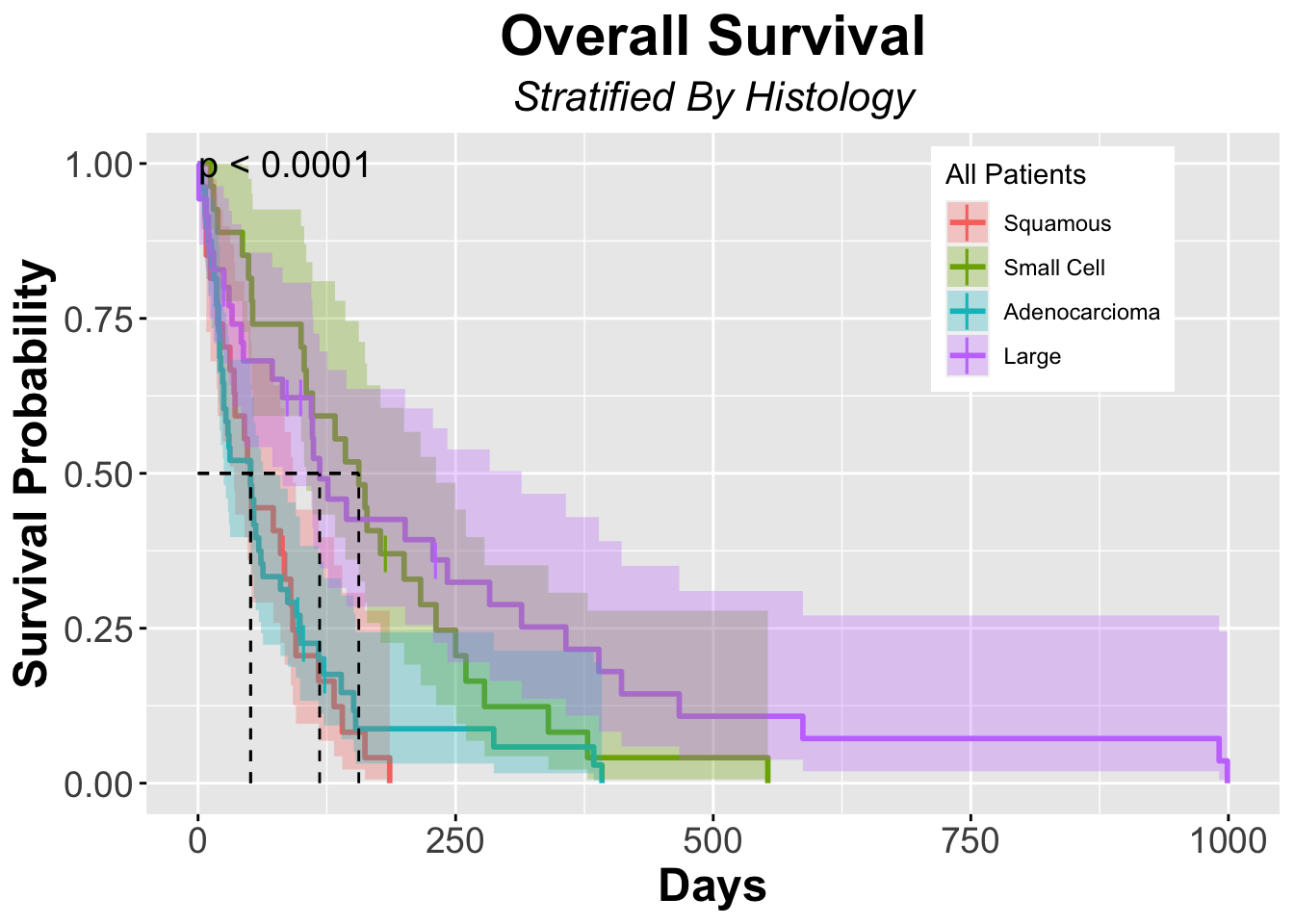
ggsurvplot(fit = veteran_Survfit_histo, 
           data = veteran,
           title = "Overall Survival",
           subtitle = "Stratified By Histology",
           font.title = c(22, "bold", "black"),
           ggtheme = theme_minimal() + theme(plot.title = element_text(hjust = 0.5, face = "bold"))+ # theme_minimal will give a white background with grid lines on the plot
             theme(plot.subtitle = element_text(hjust = 0.5, size = 16, face = "italic")),
           ####### Censor Details ########
           censor = TRUE, #ogical value. If TRUE, censors will be drawn,
           censor.shape="|",
           censor.size = 5,
           ####### Confidence Intervals ########
           conf.int = TRUE, # To Remove conf intervals use "FALSE"
           surv.median.line = "hv", # allowed values include one of c("none", "hv", "h", "v"). v: vertical, h:horizontal
           ####### Format Axes #######
           xlab="Days", # changes xlabel,
           ylab = "Survival Probability",
           font.x=c(18,"bold"), # changes x axis labels
           font.y=c(18,"bold"), # changes y axis labels
           font.xtickslab=c(14,"plain"), # changes the tick label on x axis
           font.ytickslab=c(14,"plain"),
           ######## Format Legend #######
           legend = "none",
           legend.title = "All Patients",
           legend.labs = c("Squamous","Small Cell","Adenocarcioma","Large"), # Change the Strata Legend
           ######## Plot Dimensions #######
           surv.plot.height = 0.85, # Default is 0.75
           ######## Risk Table #######
           risk.table = TRUE, # Adds Risk Table
           risk.table.height = 0.25, # Adjusts the height of the risk table (default is 0.25)
           risk.table.fontsize = 3.0)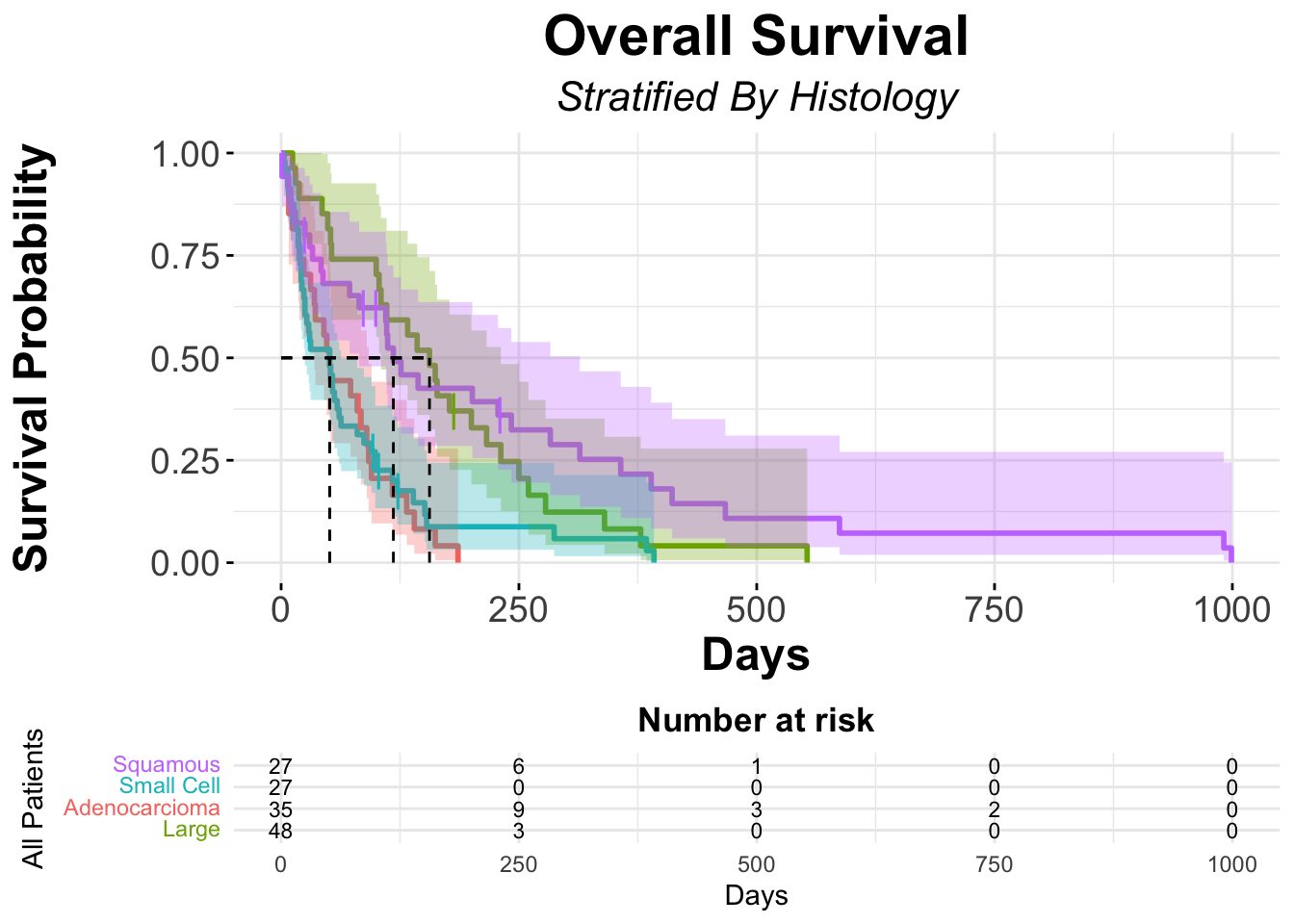

Log-Rank Analysis

Overview

To test for a difference between survival curves, we can use the survdiff() function
We specify the survival object (which contains the time-to-event and failure indicators) using the Surv command and the predictor variable
This takes the following argument structure:

survdiff(SurvObject ~ Predictor Variable, data = DataFrame)

survdiff(Surv(time = veteran$time, event = veteran$status) ~ veteran$trt, data = veteran)

Call:
survdiff(formula = Surv(time = veteran$time, event = veteran$status) ~ 
    veteran$trt, data = veteran)

               N Observed Expected (O-E)^2/E (O-E)^2/V
veteran$trt=1 69       64     64.5   0.00388   0.00823
veteran$trt=2 68       64     63.5   0.00394   0.00823

 Chisq= 0  on 1 degrees of freedom, p= 0.9

The output from the log-rank test provides important information:
- First, the output provides the observed number of events and the expected number of events under the null hypothesis of no group difference
- We can use this part of the output to determine the direction of the effect (i.e. which group had the event faster).
- In this table, we can see that both groups (trt=1) and (trt=2) were similar as expected
  - Consequently it is not surprising that the p value is close to 1 (here p = 0.9)

If we look at the log-rank for outcomes of the different cell types

survdiff(Surv(time = veteran$time, event = veteran$status) ~ veteran$celltype, data = veteran)

Call:
survdiff(formula = Surv(time = veteran$time, event = veteran$status) ~ 
    veteran$celltype, data = veteran)

                            N Observed Expected (O-E)^2/E (O-E)^2/V
veteran$celltype=squamous  35       31     47.7      5.82     10.53
veteran$celltype=smallcell 48       45     30.1      7.37     10.20
veteran$celltype=adeno     27       26     15.7      6.77      8.19
veteran$celltype=large     27       26     34.5      2.12      3.02

 Chisq= 25.4  on 3 degrees of freedom, p= 1e-05

Here we see that patients with Small Cell histology have more events than expected, meaning they did worse than expected compared to the null hypotheis.

Graph Kaplan-Meier with log-rank test displayed

ggsurvplot(fit = veteran_Survfit_histo, 
           data = veteran,
           title = "Overall Survival",
           subtitle = "Stratified By Histology",
           font.title = c(22, "bold", "black"),
           ggtheme = theme_grey() + theme(plot.title = element_text(hjust = 0.5, face = "bold"))+ # theme_grey will give a grey background with  lines on the plot
             theme(plot.subtitle = element_text(hjust = 0.5, size = 16, face = "italic")),
           ####### Censor Details ########
           censor = TRUE, #ogical value. If TRUE, censors will be drawn
           censor.shape="|",
           censor.size = 5,
           ####### Confidence Intervals ########
           conf.int = TRUE, # To Remove conf intervals use "FALSE"
           surv.median.line = "hv", # allowed values include one of c("none", "hv", "h", "v"). v: vertical, h:horizontal
           ####### Format Axes #######
           xlab="Days", # changes xlabel,
           ylab = "Survival Probability",
           font.x=c(18,"bold"), # changes x axis labels
           font.y=c(18,"bold"), # changes y axis labels
           font.xtickslab=c(14,"plain"), # changes the tick label on x axis
           font.ytickslab=c(14,"plain"),
           ######## Format Legend #######
           legend.title = "All Patients",
           legend.labs = c("Squamous","Small Cell","Adenocarcioma","Large"), # Change the Strata Legend
           legend = c(0.8,0.8), #c(0,0) corresponds to the "bottom left" and c(1,1) corresponds to the "top right" position
           ######## Plot Dimensions #######
           surv.plot.height = 0.95, # Default is 0.75
           ######## Risk Table #######
           risk.table = FALSE, # Adds Risk Table
           risk.table.height = 0.35, # Adjusts the height of the risk table (default is 0.25)
           risk.table.fontsize = 3,
           ######## p-value details #######
           pval = TRUE,
           pval.size = 5,
           pval.coord = c(1,1)
           )

Modeling Survival Data

Overview

The goal of modeling survival data is to model the relationship between survival and explanatory variables
The Cox Proportional Hazards Model is the most common model used for survival data
- It is popular because it allows for a flexible choice of covariates, it is fairly easy to fit and can be performed by standard software (including, of course, R)
- First introduced in 1972, The Cox Proportional Hazards model is a linear model for the log of the hazard ratio
- Generally speaking a “Hazard” is the probability of experiencing an event in a defined time period given that the subject has not experienced that event leading up to the interval
  - It is a “conditional” probability: i.e. the condition is that the subject in question has not yet experienced the event of interest by the beginning of the interval in question
- The Proportional Hazards (PH) models λ(t;Ζ) = λ0(t)Ψ(Ζ)
- The Cox Proportional hazards model has the advantage over a simple log-rank test of giving us an estimate of the “hazard ratio”
- This is more informative than just a test statistic, and we can also form confidence intervals for the hazard ratio

Important Caveats to Proportional Hazards Models

A condition of the Cox model is that the hazards in the groups being tested are proportional
- What this means is that from the beginning of the study period to it’s end (i.e. the completion of the follow up period) the Hazard Ratio must remain constant for the hazards to be considered proportional
- However, as summarized nicely in their article, Stensrud and Hernán point out that in clinical research, especially intervention trials, due to factors such as variations in disease susceptibility and temporally differential effects between treatment groups, Hazards are quite commonly Not Proportional
  - Given this reality, Hazard Ratios must be interpreted in their appropriate context. Stensrud and Hernán suggest ways to supplement HRs with reports of effect measures such as restricted mean survival difference
    - A detailed analysis of these approaches is beyond the scope of this post, but we encourage you to read their JAMA article and accompanied references

`R` Logistics

In R, a Cox Model takes the following form

coxph(surv(TimeVariable, EventVariable)~IndicatorVariable, data = DataFrame)

Coxph in Action

In the Veteran data set, let’s look at a model that evaluates the outcome of survival time when the Predictor is Treatment

coxph(Surv(time = veteran$time, event = veteran$status)  ~ veteran$trt, data = veteran)

Call:
coxph(formula = Surv(time = veteran$time, event = veteran$status) ~ 
    veteran$trt, data = veteran)

               coef exp(coef) se(coef)     z     p
veteran$trt 0.01774   1.01790  0.18066 0.098 0.922

Likelihood ratio test=0.01  on 1 df, p=0.9218
n= 137, number of events= 128

Interpretation:
- patients who received treatment had an increase in the log(HR) of survival by 0.01774

In the Veteran data set, let’s look at a model that evaluates the outcome of survival time when the Predictor is Cell Type

coxph(Surv(time = veteran$time, event = veteran$status)  ~ veteran$celltype, data = veteran)

Call:
coxph(formula = Surv(time = veteran$time, event = veteran$status) ~ 
    veteran$celltype, data = veteran)

                            coef exp(coef) se(coef)     z        p
veteran$celltypesmallcell 1.0013    2.7217   0.2535 3.950 7.83e-05
veteran$celltypeadeno     1.1477    3.1510   0.2929 3.919 8.90e-05
veteran$celltypelarge     0.2301    1.2588   0.2773 0.830    0.407

Likelihood ratio test=24.85  on 3 df, p=1.661e-05
n= 137, number of events= 128

Interpretation:

compared to patients with a squamous histology, for patients with small cell histology there is a increase in the log(HR) of having an event by 1.0013 (which is statisically significant)
compared to patients with a squamous histology, for patients with adenocarcinoma there is a increase in the log(HR) of having an event by 1.1477 (which is statisically significant)
compared to patients with a squamous histology, for patients with large cell histology there is a increase in the log(HR) of having an event by 0.2301 (though this is NOT statisically significant)

These results make intuitive sense. If we look at the survival curves, Large Cell Histology appears to have the best OS (MST of 156 days), meaning this is the group that has the fewest proportional events, where as both small cell and adenocarcinoma have an MST of 51 days, meaning they do worse and thus have more events

With this dataset, we can also test hypotheses based on our biological understanding of lung cancer
- For example if we wanted to test the hypothesis that the treatment tested would be effective in patients with Small Cell Lung Cancer, we could subset the data set, pulling out the patients with SCLC and perform either a log-rank test or CoxPH, as follows

SCLC <-  veteran %>% filter(celltype=="smallcell")
survdiff(Surv(time = SCLC$time, event = SCLC$status) ~ SCLC$trt, data = SCLC)

Call:
survdiff(formula = Surv(time = SCLC$time, event = SCLC$status) ~ 
    SCLC$trt, data = SCLC)

            N Observed Expected (O-E)^2/E (O-E)^2/V
SCLC$trt=1 30       28     32.3     0.575      2.28
SCLC$trt=2 18       17     12.7     1.464      2.28

 Chisq= 2.3  on 1 degrees of freedom, p= 0.1

coxph(Surv(time = SCLC$time, event = SCLC$status) ~ SCLC$trt, data = SCLC)

Call:
coxph(formula = Surv(time = SCLC$time, event = SCLC$status) ~ 
    SCLC$trt, data = SCLC)

           coef exp(coef) se(coef)     z    p
SCLC$trt 0.5020    1.6521   0.3313 1.515 0.13

Likelihood ratio test=2.24  on 1 df, p=0.1342
n= 48, number of events= 45

If we wanted to test the hypothesis that the treatment tested would be effective in patients with adenocarcinoma, we could subset the data set, pulling out the patients with adenocarcinoma and perform either a log-rank test or CoxPH, as follows

adeno <-  veteran %>% filter(celltype=="adeno")
survdiff(Surv(time = adeno$time, event = adeno$status) ~ adeno$trt, data = adeno)

Call:
survdiff(formula = Surv(time = adeno$time, event = adeno$status) ~ 
    adeno$trt, data = adeno)

             N Observed Expected (O-E)^2/E (O-E)^2/V
adeno$trt=1  9        9     10.1     0.128     0.233
adeno$trt=2 18       17     15.9     0.082     0.233

 Chisq= 0.2  on 1 degrees of freedom, p= 0.6

coxph(Surv(time = adeno$time, event = adeno$status) ~ adeno$trt, data = adeno)

Call:
coxph(formula = Surv(time = adeno$time, event = adeno$status) ~ 
    adeno$trt, data = adeno)

            coef exp(coef) se(coef)     z     p
adeno$trt 0.2067    1.2296   0.4322 0.478 0.633

Likelihood ratio test=0.23  on 1 df, p=0.6297
n= 27, number of events= 26

If we wanted to test the hypothesis that the treatment tested would be effective in patients with squamous cell carcinoma, we could subset the data set, pulling out the patients with SCC and perform either a log-rank test or CoxPH, as follows

SCC <-  veteran %>% filter(celltype=="squamous")
survdiff(Surv(time = SCC$time, event = SCC$status) ~ SCC$trt, data = SCC)

Call:
survdiff(formula = Surv(time = SCC$time, event = SCC$status) ~ 
    SCC$trt, data = SCC)

           N Observed Expected (O-E)^2/E (O-E)^2/V
SCC$trt=1 15       13     9.22     1.545      2.45
SCC$trt=2 20       18    21.78     0.655      2.45

 Chisq= 2.5  on 1 degrees of freedom, p= 0.1

coxph(Surv(time = SCC$time, event = SCC$status) ~ SCC$trt, data = SCC)

Call:
coxph(formula = Surv(time = SCC$time, event = SCC$status) ~ SCC$trt, 
    data = SCC)

           coef exp(coef) se(coef)      z     p
SCC$trt -0.6081    0.5444   0.3954 -1.538 0.124

Likelihood ratio test=2.32  on 1 df, p=0.1274
n= 35, number of events= 31

Modeling more than one predictor

Overview

The Cox Proportional Model can be used to evalute the effect of multiple Explanatory Variables (i.e Predictors) on an outcome - here survival
To do so, use the following structure
coxph(surv(TimeVariable, EventVariable) ~ IndicatorVariable1 + IndicatorVariable2 + …, data = DataFrame)
If we wanted to model the Veteran data set evaluating the effect on survival of the treatment and cell type we would use the following model

coxph(Surv(time = veteran$time, event = veteran$status)  ~ veteran$trt + veteran$celltype, data = veteran)

Call:
coxph(formula = Surv(time = veteran$time, event = veteran$status) ~ 
    veteran$trt + veteran$celltype, data = veteran)

                            coef exp(coef) se(coef)     z        p
veteran$trt               0.1978    1.2187   0.1968 1.005    0.315
veteran$celltypesmallcell 1.0964    2.9935   0.2725 4.024 5.73e-05
veteran$celltypeadeno     1.1689    3.2184   0.2950 3.962 7.43e-05
veteran$celltypelarge     0.2970    1.3459   0.2857 1.040    0.298

Likelihood ratio test=25.86  on 4 df, p=3.381e-05
n= 137, number of events= 128

If you had a biological rationale, you could build a model with all of the covariates in order to see their effect on survial, as follows:

coxph(Surv(time = veteran$time, event = veteran$status)  ~ veteran$trt + veteran$celltype + veteran$karno + veteran$diagtime + veteran$age + veteran$prior, data = veteran)

Call:
coxph(formula = Surv(time = veteran$time, event = veteran$status) ~ 
    veteran$trt + veteran$celltype + veteran$karno + veteran$diagtime + 
        veteran$age + veteran$prior, data = veteran)

                                coef  exp(coef)   se(coef)      z        p
veteran$trt                2.946e-01  1.343e+00  2.075e-01  1.419  0.15577
veteran$celltypesmallcell  8.616e-01  2.367e+00  2.753e-01  3.130  0.00175
veteran$celltypeadeno      1.196e+00  3.307e+00  3.009e-01  3.975 7.05e-05
veteran$celltypelarge      4.013e-01  1.494e+00  2.827e-01  1.420  0.15574
veteran$karno             -3.282e-02  9.677e-01  5.508e-03 -5.958 2.55e-09
veteran$diagtime           8.132e-05  1.000e+00  9.136e-03  0.009  0.99290
veteran$age               -8.706e-03  9.913e-01  9.300e-03 -0.936  0.34920
veteran$prior              7.159e-03  1.007e+00  2.323e-02  0.308  0.75794

Likelihood ratio test=62.1  on 8 df, p=1.799e-10
n= 137, number of events= 128

Review above principles with `colon` data set

The colon data set consists of data from the trials evaluating adjuvant therapy in colon cancer and is a built-in dataset within R

Definition of Variables in Colon Data Set
id: id
study: 1 for all patients
rx: Treatment - Obs(ervation), Lev(amisole), Lev(amisole)+5-FU
sex: 1=male
age: in years
obstruct: obstruction of colon by tumour
perfor: perforation of colon
adhere: adherence to nearby organs
nodes: number of lymph nodes with detectable cancer
time: days until event or censoring
status: censoring status
differ: differentiation of tumour (1=well, 2=moderate, 3=poor)
extent: Extent of local spread (1=submucosa, 2=muscle, 3=serosa, 4=contiguous structures)
surg: time from surgery to registration (0=short, 1=long)
node4: more than 4 positive lymph nodes
etype: event type: 1=recurrence,2=death

Note: The study is originally described in a 1989 Journal of Clinical Oncology paper by Laurie et al. The main report is found in a 1990 New England Journal of Medicine paper by Moertel et al. This data set, which is contained in R, is closest to that of the final report in the 1991 Annals of Internal Medicine paper by Moertel et al. A version of the data with less follow-up time was used in the paper in Statistics in Medicine by Lin (1994).

References

JA Laurie, CG Moertel, TR Fleming, HS Wieand, JE Leigh, J Rubin, GW McCormack, JB Gerstner, JE Krook and J Malliard. Surgical adjuvant therapy of large-bowel carcinoma: An evaluation of levamisole and the combination of levamisole and fluorouracil: The North Central Cancer Treatment Group and the Mayo Clinic. J Clinical Oncology, 7:1447-1456, 1989.

DY Lin. Cox regression analysis of multivariate failure time data: the marginal approach. Statistics in Medicine, 13:2233-2247, 1994.

CG Moertel, TR Fleming, JS MacDonald, DG Haller, JA Laurie, PJ Goodman, JS Ungerleider, WA Emerson, DC Tormey, JH Glick, MH Veeder and JA Maillard. Levamisole and fluorouracil for adjuvant therapy of resected colon carcinoma. New England J of Medicine, 332:352-358, 1990.

CG Moertel, TR Fleming, JS MacDonald, DG Haller, JA Laurie, CM Tangen, JS Ungerleider, WA Emerson, DC Tormey, JH Glick, MH Veeder and JA Maillard, Fluorouracil plus Levamisole as an effective adjuvant therapy after resection of stage II colon carcinoma: a final report. Annals of Internal Med, 122:321-326, 1991.

View Head of Data Set

kable(head(colon))

id	study	rx	sex	age	adhere	nodes	status	differ	extent	node4	time	etype
1	1	Lev+5FU	1	43	0	5	1	2	3	1	1521	2
1	1	Lev+5FU	1	43	0	5	1	2	3	1	968	1
2	1	Lev+5FU	1	63	0	1	0	2	3	0	3087	2
2	1	Lev+5FU	1	63	0	1	0	2	3	0	3087	1
3	1	Obs	0	71	1	7	1	2	2	1	963	2
3	1	Obs	0	71	1	7	1	2	2	1	542	1

Kaplan-Meier Curve of the colon data set

colon_Survfit <- survfit(Surv(time = colon$time, event = colon$status) ~ 1, data = colon)
colon_ggSurvplot <- ggsurvplot (fit = colon_Survfit, 
           data = colon,
           title = "Overall Survival",
           subtitle = "Unstratified Curve",
           font.title = c(22, "bold", "black"),
           ggtheme = theme_dark() + theme(plot.title = element_text(hjust = 0.5, face = "bold"))+
             # theme_dark will give a dark background with lines on the plot
             theme(plot.subtitle = element_text(hjust = 0.5, size = 16, face = "italic")),
           ####### Censor Details ########
           censor = TRUE, # logical value. If TRUE, censors will be drawn
           censor.shape="|",
           censor.size = 5,
           ####### Confidence Intervals ########
           conf.int = TRUE, # To Remove conf intervals use "FALSE"
           surv.median.line = "hv", # allowed values include one of c("none", "hv", "h", "v"). v: vertical, h:horizontal
           ####### Format Axes #######
           xlab="Days", # changes xlabel,
           ylab = "Survival Probability",
           font.x=c(18,"bold"), # changes x axis labels
           font.y=c(18,"bold"), # changes y axis labels
           font.xtickslab=c(14,"plain"), # changes the tick label on x axis
           font.ytickslab=c(14,"plain"),
           ######## Format Legend #######
           legend.title = "All Patients",
           legend.labs = c("Total Cohort"), # Change the Strata Legend
           legend = c(0.8,0.8), #c(0,0) corresponds to the "bottom left" and c(1,1) corresponds to the "top right" position
           ######## Plot Dimensions #######
           surv.plot.height = 0.75, # Default is 0.75
           ######## Risk Table #######
           risk.table = FALSE, # Adds Risk Table
           risk.table.height = 0.35, # Adjusts the height of the risk table (default is 0.25)
           ######## p-value details #######
           pval = FALSE,
           pval.size = 5,
           pval.coord = c(1,1)
           )
colon_ggSurvplot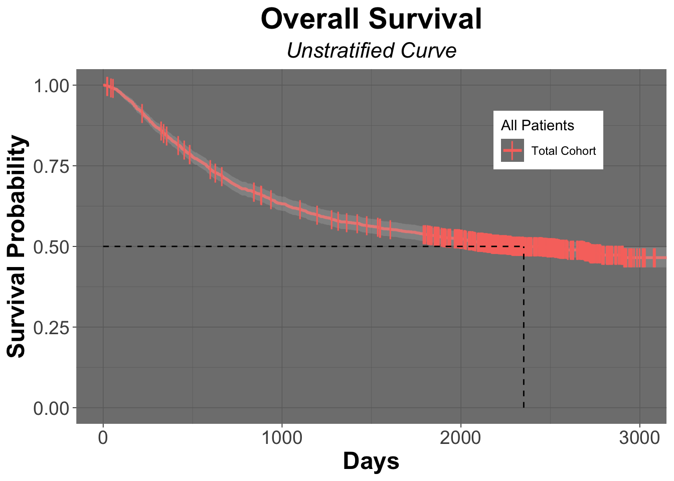

View Kaplan-Meier Curve of Cohort Stratified by Treatment

First let’s generate a survfit object of the data stratified by treatment

colon_Survfit_rx <- survfit(Surv(time = colon$time, event = colon$status) ~ colon$rx, data = colon)

Let’s now view that survfit object

colon_Survfit_rx

Call: survfit(formula = Surv(time = colon$time, event = colon$status) ~ 
    colon$rx, data = colon)

                   n events median 0.95LCL 0.95UCL
colon$rx=Obs     630    345   1723    1323    2213
colon$rx=Lev     620    333   1709    1219    2593
colon$rx=Lev+5FU 608    242     NA      NA      NA

From the above table, it appears like the group of patients that received Levamisole (Lev) and 5-FU in the adjuvant setting had fewer events than those in the observation group or the levamisole only group.

To evaluate if what we observed is different from what we’d expect under the null hypothesis, let’s evaluate using the log-rank test

survdiff(Surv(time, status) ~ rx, data = colon)# of note, you'll see that we used a slightly different way to write the above code. It's a simpler way in which we only use the column names and do not require the preceeding "colon$", which is actually not needed, since we are specifying the data set

Call:
survdiff(formula = Surv(time, status) ~ rx, data = colon)

             N Observed Expected (O-E)^2/E (O-E)^2/V
rx=Obs     630      345      299      7.01     10.40
rx=Lev     620      333      295      4.93      7.26
rx=Lev+5FU 608      242      326     21.61     33.54

 Chisq= 33.6  on 2 degrees of freedom, p= 5e-08

As you can see from the above table, there are indeed much fewer events in the Lev+5FU group than what we’d expect under the null, and it is statistically significant

Now we will generate a Kaplan-Meier curve of those three groups

colon_ggSurvplot_rx <- ggsurvplot (fit = colon_Survfit_rx, 
           data = colon,
           title = "Overall Survival",
           subtitle = "Stratified by Treatment Group",
           font.title = c(22, "bold", "black"),
           ggtheme = theme_minimal() + theme(plot.title = element_text(hjust = 0.5, face = "bold"))+
             theme(plot.subtitle = element_text(hjust = 0.5, size = 16, face = "italic")),
           ####### Censor Details ########
           censor = TRUE, # logical value. If TRUE, censors will be drawn
           censor.shape="|",
           censor.size = 5,
           ####### Confidence Intervals ########
           conf.int = TRUE, # To Remove conf intervals use "FALSE"
           surv.median.line = "hv", # allowed values include one of c("none", "hv", "h", "v"). v: vertical, h:horizontal
           ####### Format Axes #######
           xlab="Days", # changes xlabel,
           ylab = "Survival Probability",
           font.x=c(18,"bold"), # changes x axis labels
           font.y=c(18,"bold"), # changes y axis labels
           font.xtickslab=c(14,"plain"), # changes the tick label on x axis
           font.ytickslab=c(14,"plain"),
           ######## Format Legend #######
           legend.title = "All Patients",
           legend.labs = c("Observation","Levamisole","Levamisole + 5-FU"), # Change the Strata Legend
           legend = c(0.8,0.8), #c(0,0) corresponds to the "bottom left" and c(1,1) corresponds to the "top right" position
           ######## Plot Dimensions #######
           surv.plot.height = 0.75, # Default is 0.75
           ######## Risk Table #######
           risk.table = FALSE, # Adds Risk Table
           risk.table.height = 0.35, # Adjusts the height of the risk table (default is 0.25)
           ######## p-value details #######
           pval = TRUE,
           pval.size = 5,
           pval.coord = c(1,0.1)
           )
colon_ggSurvplot_rx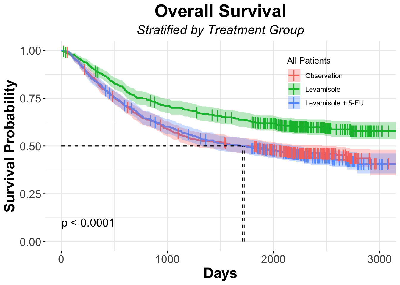

Visualize Hazard Ratios with Forest Plots

Overview

Forest plots allow you to evaluate the Hazard Ratios (HR) of all of the covariates that were used in the model you created
Let’s build a model incorporating covariates that think might influence or explain (i.e. explanatory variables) the survival curve, such as age, treatment, whether or not the tumor adhered to other organs or if patients had more than 4 nodes positive, differentiation status of the tumor, the extent of local spread and time from surgery to registration
- Biologically, all of these covariates may effect the outcome, so you might want to include them in your model

model.colon <- coxph( Surv(time, status) ~ sex + rx + adhere + node4 + extent + surg + differ,
                data = colon )
model.colon # Call the model to inspect it's contents

Call:
coxph(formula = Surv(time, status) ~ sex + rx + adhere + node4 + 
    extent + surg + differ, data = colon)

              coef exp(coef) se(coef)      z        p
sex       -0.04499   0.95601  0.06706 -0.671 0.502361
rxLev     -0.01322   0.98687  0.07836 -0.169 0.866068
rxLev+5FU -0.42424   0.65427  0.08466 -5.011 5.42e-07
adhere     0.16073   1.17437  0.08991  1.788 0.073832
node4      0.84508   2.32818  0.06921 12.210  < 2e-16
extent     0.43480   1.54466  0.08098  5.369 7.90e-08
surg       0.24756   1.28089  0.07288  3.397 0.000682
differ     0.19508   1.21541  0.06839  2.853 0.004337

Likelihood ratio test=249.3  on 8 df, p=< 2.2e-16
n= 1812, number of events= 899 
   (46 observations deleted due to missingness)

From the above table, you see that there are a number of covariates that appear to be related to the survival outcome (here recurrence or death). - The column exp(coef) represents the “Hazard Ratio”, which is the most common way to compare the relationship between an explanatory variable and the outcome variable in medical research
- A HR of 1 is the null hypothesis
- A HR < 1 means that there is a decreased risk of the outcome (in survival analysis this = death) if that specific condition is met by the subject (i.e. they received the treatment)
- A HR > 1 means that there is an increased risk of the outcome (in survival analysis this = death) if that specific condition is met by the subject (i.e. had more than 4 positive lymph nodes)

Let’s view the Forest Plot of that model

ggforest(model.colon)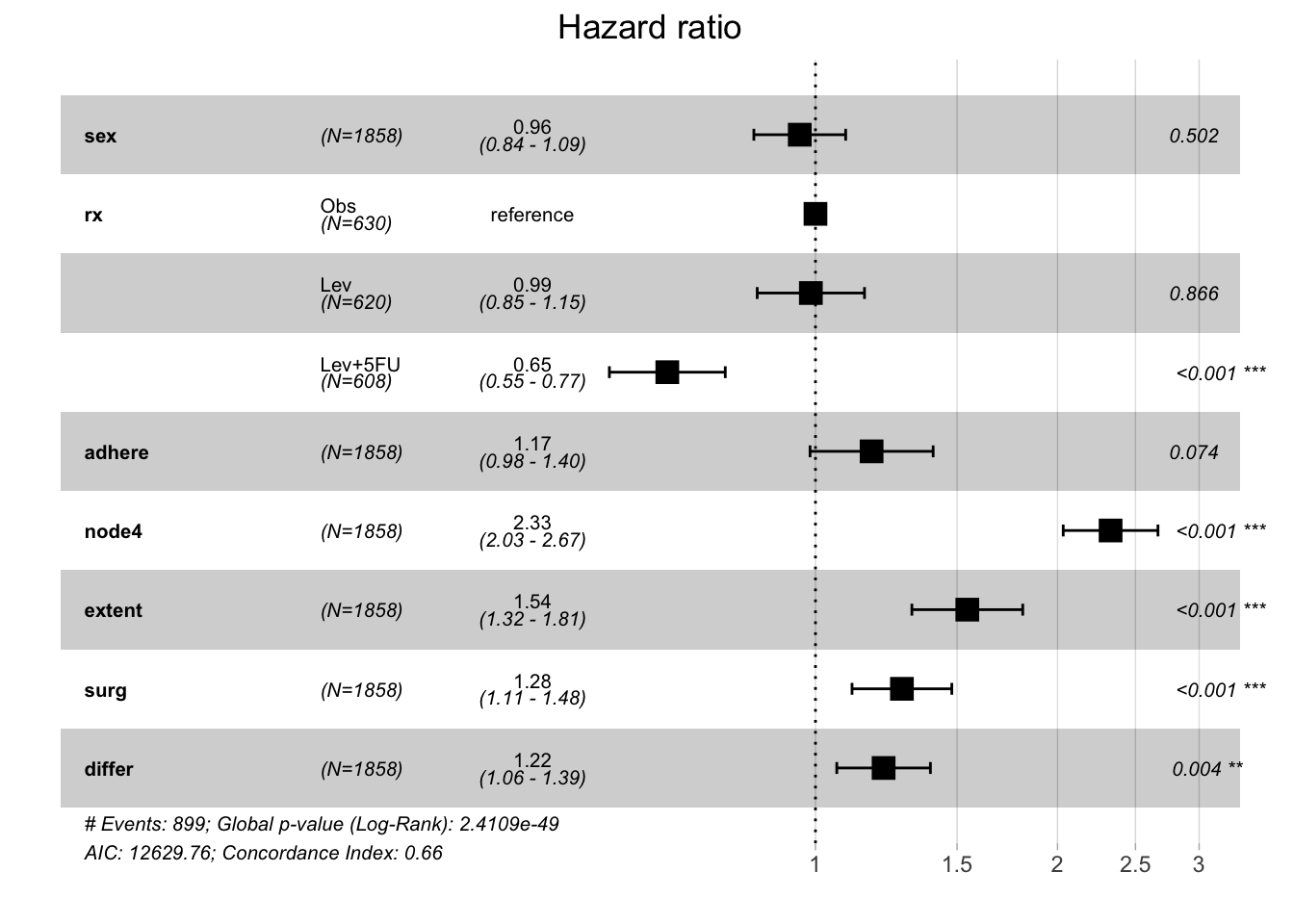

Interpretation from this model could be the following:
- There is no difference in death between males and females
- Treatment with Lev+5FU in this cohort is associated with a 35% decreased risk of recurrence or death compared to subjects that received only observation
- There is a trend to worse outcomes in patients tumors that adhere to nearby organs
- Worse outcomes are associated with more than 4 positive lymph nodes, extention of the tumor, long times between surgery and registration to the trial and poorly differentiated tumors.

Of note, you’ll see that your HRs will change depending on what covariates you include in your model. For example your interpretation of whether or not adherence to the surrounding tissue is associated with worse outcomes will be affected by the covariate you include in the model. Watch what happens if we leave “node4”, “extent” and “differ” out of the model

model.colon <- coxph( Surv(time, status) ~ sex + rx + adhere  + surg,
                data = colon )
ggforest(model.colon)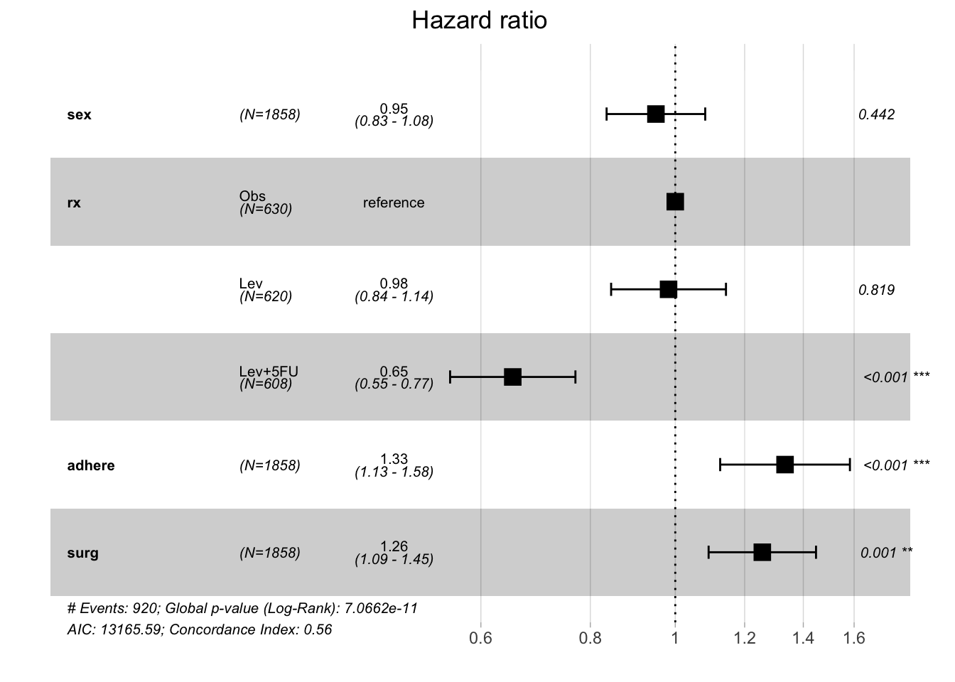

Now it appears that adherence to organs is indeed associated with worse outcomes with a p-value <0.001), whereas in the first model the p-value of this covariate trended towards statistical significance but the 95% CI overlapped the null and therefore, rejecting the null would have been in appropriate

This brings up a critical principle in science.

You must be very rigorous about your hypothesis testing and prespecify which hypotheses you are going to test before you analyze your data
What can be tempting - but is inappropriate - is to look at your data from numerous viewpoints, testing one hypothesis in sequence after another in order to find a statistically significant p value
This practice is probably more common in science than we would like to acknowledge and can lead to inappropriate rejection of the null hypothesis
- This methodology has many pejorative sobriquets including “data dredging”, “data fishing”, “data butchery” or “p-hacking”
- This highlights the need to be very thoughtful about your analysis upfront
  - Consulting a biostatistician before carrying out your analysis is ideal
  - In fact, consulting one before conducting your research, so you can have a Statistical Analysis Plan before you conduct your research, is part-and-parcel with good science

Conclusion

Survival Analyses are some of the most common analysis in clinical research
R has several nice packages that can faciliate Survival Analysis
Beware of “p-hacking”: when in doubt, consult a biostatistician before you conduct your science!

As always, please reach out to us with thoughts and feedback

Session Info

sessionInfo()

R version 4.2.0 (2022-04-22)
Platform: x86_64-apple-darwin17.0 (64-bit)
Running under: macOS Big Sur/Monterey 10.16

Matrix products: default
BLAS:   /Library/Frameworks/R.framework/Versions/4.2/Resources/lib/libRblas.0.dylib
LAPACK: /Library/Frameworks/R.framework/Versions/4.2/Resources/lib/libRlapack.dylib

locale:
[1] en_US.UTF-8/en_US.UTF-8/en_US.UTF-8/C/en_US.UTF-8/en_US.UTF-8

attached base packages:
[1] stats     graphics  grDevices utils     datasets  methods   base     

other attached packages:
 [1] survminer_0.4.9 ggpubr_0.4.0    knitr_1.41      forcats_0.5.2  
 [5] stringr_1.5.0   dplyr_1.0.10    purrr_0.3.5     readr_2.1.3    
 [9] tidyr_1.2.1     tibble_3.1.8    ggplot2_3.4.0   tidyverse_1.3.2
[13] survival_3.4-2  devtools_2.4.3  usethis_2.1.6  

loaded via a namespace (and not attached):
 [1] ggtext_0.1.1        fs_1.5.2            lubridate_1.9.0    
 [4] httr_1.4.4          rprojroot_2.0.3     tools_4.2.0        
 [7] backports_1.4.1     utf8_1.2.2          R6_2.5.1           
[10] DBI_1.1.3           colorspace_2.0-3    withr_2.5.0        
[13] gridExtra_2.3       tidyselect_1.2.0    prettyunits_1.1.1  
[16] processx_3.8.0      curl_4.3.3          compiler_4.2.0     
[19] cli_3.4.1           rvest_1.0.3         xml2_1.3.3         
[22] desc_1.4.1          labeling_0.4.2      scales_1.2.1       
[25] survMisc_0.5.6      callr_3.7.3         digest_0.6.30      
[28] rmarkdown_2.18      pkgconfig_2.0.3     htmltools_0.5.3    
[31] sessioninfo_1.2.2   highr_0.9           dbplyr_2.2.1       
[34] fastmap_1.1.0       htmlwidgets_1.5.4   rlang_1.0.6        
[37] readxl_1.4.1        rstudioapi_0.14     farver_2.1.1       
[40] generics_0.1.3      zoo_1.8-10          jsonlite_1.8.4     
[43] car_3.0-13          googlesheets4_1.0.1 magrittr_2.0.3     
[46] Matrix_1.4-1        Rcpp_1.0.9          munsell_0.5.0      
[49] fansi_1.0.3         abind_1.4-5         lifecycle_1.0.3    
[52] stringi_1.7.8       yaml_2.3.6          carData_3.0-5      
[55] brio_1.1.3          pkgbuild_1.3.1      grid_4.2.0         
[58] crayon_1.5.2        lattice_0.20-45     cowplot_1.1.1      
[61] haven_2.5.1         splines_4.2.0       gridtext_0.1.4     
[64] hms_1.1.2           ps_1.7.2            pillar_1.8.1       
[67] markdown_1.1        ggsignif_0.6.3      pkgload_1.2.4      
[70] reprex_2.0.2        glue_1.6.2          evaluate_0.18      
[73] data.table_1.14.6   remotes_2.4.2       modelr_0.1.10      
[76] vctrs_0.5.1         tzdb_0.3.0          testthat_3.1.4     
[79] cellranger_1.1.0    gtable_0.3.1        km.ci_0.5-6        
[82] assertthat_0.2.1    cachem_1.0.6        xfun_0.35          
[85] xtable_1.8-4        broom_1.0.1         rstatix_0.7.0      
[88] googledrive_2.0.0   gargle_1.2.1        KMsurv_0.1-5       
[91] memoise_2.0.1       timechange_0.1.1    ellipsis_0.3.2

Key points

Background on Survival Analysis

Handling Dates

Load Packages and Data Sets

Load the survival package

Load Other Packages

Load Data Sets

Overview

Kaplan-Meier Estimator

Overview

Analyze Survival Data in R

Surv() Function

Build Surv Object

Analyze the Survival Data with the survfit() function

Generate a KM Curve

Overview

Visualizing Survival Data

Overview

Plot Data Using Base R

Plot Data Using ggsurvplot

KM Curves with a Predictor

Overview

Stratify Analysis Based on Treatment (Standard vs. Experimental)

Another Example of a KM stratified by an Explanatory Variable - Cell Type

Log-Rank Analysis

Overview

Graph Kaplan-Meier with log-rank test displayed

Modeling Survival Data

Overview

Important Caveats to Proportional Hazards Models

R Logistics

Coxph in Action

Modeling more than one predictor

Overview

Review above principles with colon data set

View Head of Data Set

Kaplan-Meier Curve of the colon data set

View Kaplan-Meier Curve of Cohort Stratified by Treatment

Visualize Hazard Ratios with Forest Plots

Overview

This brings up a critical principle in science.

Conclusion

Session Info

Load the `survival` package

`Surv()` Function

Analyze the Survival Data with the `survfit()` function

Plot Data Using Base `R`

Plot Data Using `ggsurvplot`

`R` Logistics

Review above principles with `colon` data set