library(ggplot2)
library(dplyr, warn.conflicts=FALSE)   # Useful for manipulating the dataframes
library(reshape2) # Reformmating dataframes
library(grid)
library(plotly) # Allows us to make the swimmer plot interactive
library(knitr)Graphical Representation of Survival - Swimmer Plots for Clinical Trials in Clinical Oncology
Abstract
In this post we demonstrate how to create Swimmer Plots to visualize Survival Data in R
Overview
- This is an RMarkdown explaining how we can use “Swimmer Plots” to visualize survival data.
- A “Swimmer Plot” is a graphical way of displaying several aspects of a subject’s tumor response such as total time to tumor response, whether there was a “Complete” or “Partial” response, and duration of response.
- This is a clear, graphical representation of the course of a patient’s tumor response and can be an especially useful tool when reporting clinical trial data results.
Prepare the Data
Step 1, Download ggplot2, reshape2, dplyr, plotly, and grid from CRAN
- Use the
install.package()function to install the followng R packages from CRAN:ggplot2,plotly,reshape2,dplyr,kintrandgridfrom CRAN for example:
install.packages("ggplot2")
Step 2, Load each relevant Package
Step 3, Create an “example” data set for demonstrative purposes
- We will create a working data set appropriate for this type of graphical represenataion.
set.seed(35) # This sets the seed of R's random number generator
dat <-  data.frame(Subject = 1:15,
                 Months = sample(5:20, 15, replace=TRUE), # This generates a random set of months from 5 - 20
                 Treated=sample(0:1, 15, replace=TRUE), # This generates 15 random 0 or 1s which correspond to Tx or no Tx
                 Stage = sample(1:4, 15, replace=TRUE), # This randomly generates staging from 1 - 4
                 Continued=sample(0:15, 15, replace=TRUE))
View initial Data Set
dat %>% kable| Subject | Months | Treated | Stage | Continued |
|---|---|---|---|---|
| 1 | 14 | 0 | 4 | 5 |
| 2 | 10 | 0 | 2 | 9 |
| 3 | 12 | 0 | 1 | 0 |
| 4 | 5 | 0 | 1 | 14 |
| 5 | 11 | 0 | 2 | 10 |
| 6 | 15 | 1 | 4 | 1 |
| 7 | 13 | 0 | 1 | 13 |
| 8 | 18 | 1 | 1 | 9 |
| 9 | 9 | 0 | 2 | 0 |
| 10 | 6 | 0 | 4 | 6 |
| 11 | 6 | 0 | 3 | 2 |
| 12 | 20 | 0 | 1 | 15 |
| 13 | 13 | 0 | 2 | 2 |
| 14 | 14 | 1 | 1 | 12 |
| 15 | 13 | 0 | 1 | 0 |
Add Response Data to Data Set
dat <-  dat %>%
  group_by(Subject) %>%
  mutate(Complete=sample(c(4:(max(Months)-1),NA), 1,
                         prob=c(rep(1, length(4:(max(Months)-1))),5), replace=TRUE),
         Partial=sample(c(4:(max(Months)-1),NA), 1,
                        prob=c(rep(1, length(4:(max(Months)-1))),5), replace=TRUE),
         Durable=sample(c(-0.5,NA), 1, replace=TRUE))
# of note, `sample()`takes a sample of the specified size from the elements of x using either with or without replacement
# Let's organize the order of the Subjects by Months
dat$Subject <-  factor(dat$Subject, levels=dat$Subject[order(dat$Months)])
Let’s view the Data Set Now
dat %>% kable| Subject | Months | Treated | Stage | Continued | Complete | Partial | Durable |
|---|---|---|---|---|---|---|---|
| 1 | 14 | 0 | 4 | 5 | 5 | 11 | NA |
| 2 | 10 | 0 | 2 | 9 | NA | 4 | -0.5 |
| 3 | 12 | 0 | 1 | 0 | 5 | 8 | -0.5 |
| 4 | 5 | 0 | 1 | 14 | NA | NA | NA |
| 5 | 11 | 0 | 2 | 10 | 5 | NA | -0.5 |
| 6 | 15 | 1 | 4 | 1 | 6 | 6 | -0.5 |
| 7 | 13 | 0 | 1 | 13 | 11 | 10 | -0.5 |
| 8 | 18 | 1 | 1 | 9 | 15 | 10 | NA |
| 9 | 9 | 0 | 2 | 0 | NA | 6 | -0.5 |
| 10 | 6 | 0 | 4 | 6 | NA | NA | -0.5 |
| 11 | 6 | 0 | 3 | 2 | 4 | NA | -0.5 |
| 12 | 20 | 0 | 1 | 15 | 11 | NA | NA |
| 13 | 13 | 0 | 2 | 2 | 8 | 9 | -0.5 |
| 14 | 14 | 1 | 1 | 12 | 13 | 13 | NA |
| 15 | 13 | 0 | 1 | 0 | NA | NA | -0.5 |
Melt part of data frame for adding points to bars
- This will collapse the Columns “Complete”, “Partial” and “Durable” into a new column called “variable” and the values of those orginial columns will become a new vector/column called “value”
dat.m <-  melt(dat %>% select(Subject, Months, Complete, Partial, Durable),
             id.var=c("Subject","Months"), na.rm = TRUE)
# of note, na.rm = TRUE will eliminate those rows with missing values
Let’s View our Data Set after melting
dat.m %>% kable| Subject | Months | variable | value | |
|---|---|---|---|---|
| 1 | 1 | 14 | Complete | 5.0 |
| 3 | 3 | 12 | Complete | 5.0 |
| 5 | 5 | 11 | Complete | 5.0 |
| 6 | 6 | 15 | Complete | 6.0 |
| 7 | 7 | 13 | Complete | 11.0 |
| 8 | 8 | 18 | Complete | 15.0 |
| 11 | 11 | 6 | Complete | 4.0 |
| 12 | 12 | 20 | Complete | 11.0 |
| 13 | 13 | 13 | Complete | 8.0 |
| 14 | 14 | 14 | Complete | 13.0 |
| 16 | 1 | 14 | Partial | 11.0 |
| 17 | 2 | 10 | Partial | 4.0 |
| 18 | 3 | 12 | Partial | 8.0 |
| 21 | 6 | 15 | Partial | 6.0 |
| 22 | 7 | 13 | Partial | 10.0 |
| 23 | 8 | 18 | Partial | 10.0 |
| 24 | 9 | 9 | Partial | 6.0 |
| 28 | 13 | 13 | Partial | 9.0 |
| 29 | 14 | 14 | Partial | 13.0 |
| 32 | 2 | 10 | Durable | -0.5 |
| 33 | 3 | 12 | Durable | -0.5 |
| 35 | 5 | 11 | Durable | -0.5 |
| 36 | 6 | 15 | Durable | -0.5 |
| 37 | 7 | 13 | Durable | -0.5 |
| 39 | 9 | 9 | Durable | -0.5 |
| 40 | 10 | 6 | Durable | -0.5 |
| 41 | 11 | 6 | Durable | -0.5 |
| 43 | 13 | 13 | Durable | -0.5 |
| 45 | 15 | 13 | Durable | -0.5 |
Graph the Data using a Swimmer Plot
Let’s make a static swimmer plot with ggplot
a<- ggplot(dat, aes(Subject, Months)) +
  geom_bar(stat="identity", aes(fill=factor(Stage)), width=0.8) +
  geom_point(data=dat.m,
             aes(Subject, value, colour=variable, shape=variable), size=5) +
  geom_segment(data=dat %>% filter(Continued==1),
             aes(x=Subject, xend=Subject, y=Months + 0.1, yend=Months + 1),
             pch=15, size=0.8, arrow=arrow(type="closed", length=unit(0.1,"in"))) +
  coord_flip() +
  scale_fill_manual(values=hcl(seq(15,375,length.out=5)[1:4],100,75)) +
  scale_colour_manual(values=c(hcl(seq(15,375,length.out=3)[1:2],100,30),"black")) +
  scale_y_continuous(limits=c(-1,20), breaks=0:20) +
  labs(fill="Disease Stage", colour="", shape="",
       x="Subjects on Treatment Drug A") +
  theme_bw() +
  theme(panel.grid.minor=element_blank(),
        panel.grid.major=element_blank(),
        axis.text.y=element_blank(),
        axis.ticks.y=element_blank())
a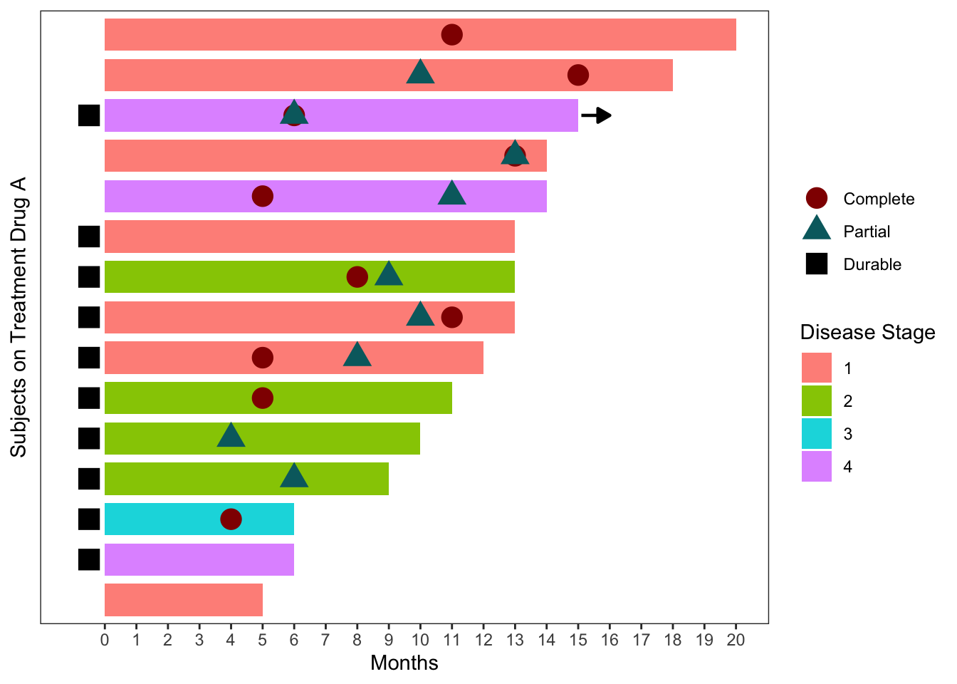
Now let’s make an Interactive Swimmer plot in Plotly by simply using the ggplotly() function of the static plot as an object
ggplotly(a)SessionInfo
sessionInfo()R version 4.2.0 (2022-04-22)
Platform: x86_64-apple-darwin17.0 (64-bit)
Running under: macOS Big Sur/Monterey 10.16
Matrix products: default
BLAS: /Library/Frameworks/R.framework/Versions/4.2/Resources/lib/libRblas.0.dylib
LAPACK: /Library/Frameworks/R.framework/Versions/4.2/Resources/lib/libRlapack.dylib
locale:
[1] en_US.UTF-8/en_US.UTF-8/en_US.UTF-8/C/en_US.UTF-8/en_US.UTF-8
attached base packages:
[1] grid stats graphics grDevices utils datasets methods
[8] base
other attached packages:
[1] knitr_1.41 plotly_4.10.1.9000 reshape2_1.4.4 dplyr_1.0.10
[5] ggplot2_3.4.0
loaded via a namespace (and not attached):
[1] Rcpp_1.0.9 highr_0.9 plyr_1.8.7 pillar_1.8.1
[5] compiler_4.2.0 tools_4.2.0 digest_0.6.30 viridisLite_0.4.1
[9] jsonlite_1.8.4 evaluate_0.18 lifecycle_1.0.3 tibble_3.1.8
[13] gtable_0.3.1 pkgconfig_2.0.3 rlang_1.0.6 cli_3.4.1
[17] DBI_1.1.3 rstudioapi_0.14 crosstalk_1.2.0 yaml_2.3.6
[21] xfun_0.35 fastmap_1.1.0 httr_1.4.4 withr_2.5.0
[25] stringr_1.5.0 generics_0.1.3 vctrs_0.5.1 htmlwidgets_1.5.4
[29] tidyselect_1.2.0 data.table_1.14.6 glue_1.6.2 R6_2.5.1
[33] fansi_1.0.3 rmarkdown_2.18 farver_2.1.1 tidyr_1.2.1
[37] purrr_0.3.5 magrittr_2.0.3 scales_1.2.1 htmltools_0.5.3
[41] assertthat_0.2.1 colorspace_2.0-3 utf8_1.2.2 stringi_1.7.8
[45] lazyeval_0.2.2 munsell_0.5.0