library(flexdashboard)
library(RCurl)
library(REDCapR)
library(httr)
library(tidyverse)
library(knitr)
library(plotly)
library(readxl)
library(scales)
library(cowplot)FlexDashboards for Clinical and Translational Research
Abstract
A monograph on how to create Dashboards using R via a package called flexdashboard
Key Points
This monograph provides a roadmap to create a FlexDashboard for Clinical and Translational Research
The purpose of a Dashboard is to present data in a way that enhances its interpretation
There are many excellent tutorials on using the package Flexdashboard to create a dashboard; however, in this monograph we aim to highlight a few pearls that we have learned along the way that we hope you’ll find useful
What we will show you next is the code we used to create the following Flexdashboard
Click here to see the interactive Dashboard
Of note, the data here is completely fabricated, any relation to real subjects is completely coincidental
Skill Level: Intermediate
- Assumption made by this post is that readers will have basic familiarity with
R
- Assumption made by this post is that readers will have basic familiarity with
Load Packages
- We will be making use of the following packages
Overview of the Format of Flexdashboard
- The
Flexdashboardpackage is built aroundRMarkdown
- To start, you can open a new RMarkdown by:
File -> New File -> RMarkdown
- Then go to “From Template” on the left hand column
- If you have installed
Flexdashboardthen Flexdashboard will be in the window that opens
- Once you have selected Flexdashboard a new RMarkdown will open
- What is specific here is the YAML
- The content between the three dashes in beginning of the RMarkdown
- If you have installed
Flexdashboard YAML
- This is the YAML for the Flexdashboard
title: “Untitled”
output:
flexdashboard::flex_dashboard:
orientation: columns
vertical_layout: fill
Flexdashboard content
- Then after the YAML, the Flexdashboard template is quite basic
- It is broken down into three basic sections, which are designated by either hashtags or dashes
Key Structure of FLEXDASHBOARD
#Page (Level 1 Header)##Column vs. Tabset (Level 2 Header)###Individual Data Visualizations (Level 3 Header)
Level 1 or The “Page” designation
- This can either be marked by a single # or by a double line ============ under the corresponding text
The Column vs. Tabset
- This can be designed by two #s (##) or a single dash line ———– under the text
The Individual Data Visualizations
- Marked by three #s (###)
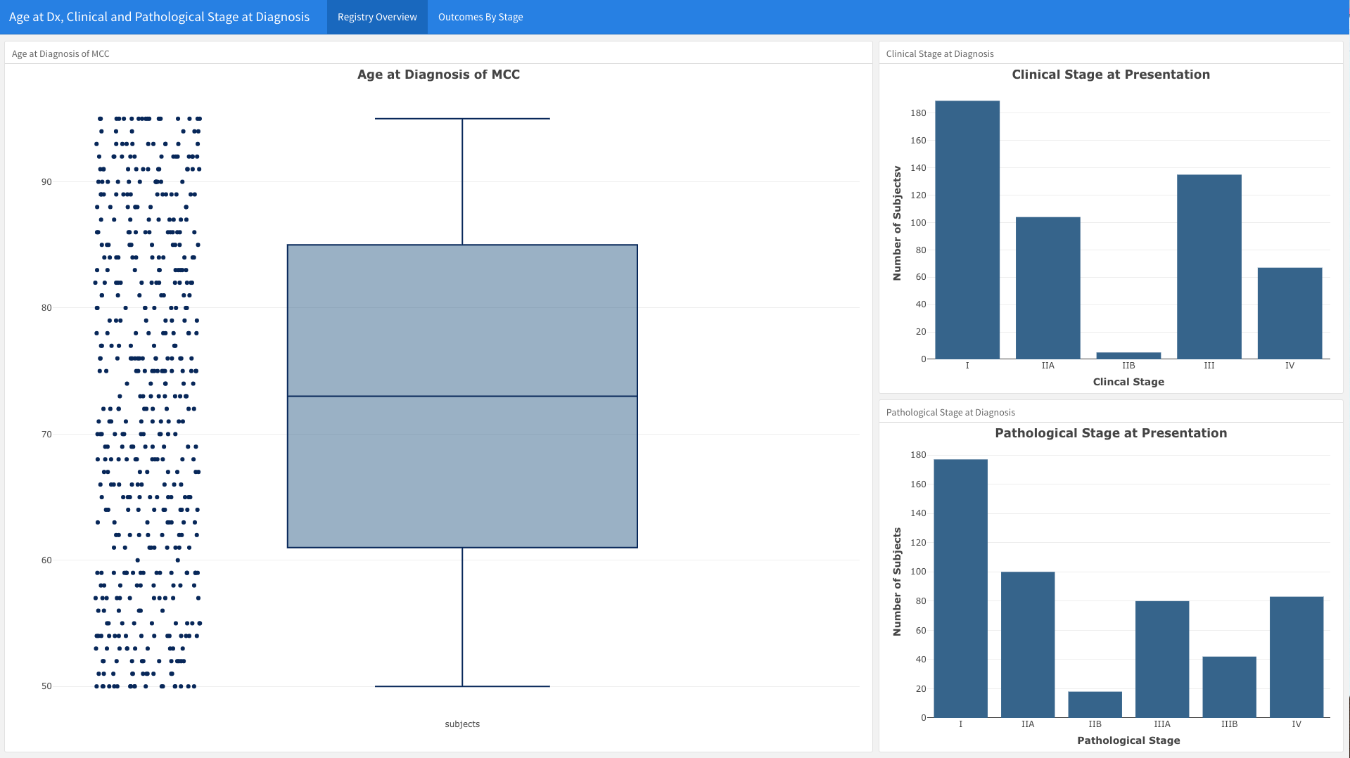
As example, using our dashboard above, we broke the first Page “Registry Overview” down into three graphs using the following structure
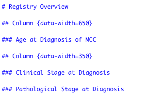
Here’s an example of what that code looks like to generate the data in the Flexdashboard
To start, let’s load the data we used
- This is a fabricated dataset, but has many features that resemble an actual rare disease cohort dataset.
dt <- data.frame(record_id = 1:500,
                 age_at_dx = sample(50:95, size = 500, replace = TRUE),
                 man_clinstage = sample(1:5, size = 500, replace = TRUE, prob = c(0.39, 0.2, 0.01, 0.25, 0.15)),
                 man_pathstage = sample(1:6, size = 500, replace = TRUE, prob = c(0.37, 0.2, 0.03, 0.15, 0.1, 0.15)),
                 overall_survival = sample(1:3000, size = 500, replace = TRUE),
                 subject_status = sample(0:1, size = 500, replace = TRUE))
View Dataset
dt %>%
  kable %>%
  kableExtra::kable_styling(bootstrap_options = c("hover","striped"),
                            fixed_thead = T) %>%
  kableExtra::scroll_box(height = "400px",
width = "100%")| record_id | age_at_dx | man_clinstage | man_pathstage | overall_survival | subject_status |
|---|---|---|---|---|---|
| 1 | 67 | 5 | 2 | 1650 | 0 |
| 2 | 81 | 2 | 1 | 1724 | 1 |
| 3 | 58 | 2 | 4 | 617 | 0 |
| 4 | 56 | 2 | 6 | 2141 | 1 |
| 5 | 73 | 1 | 6 | 361 | 1 |
| 6 | 77 | 5 | 2 | 1443 | 1 |
| 7 | 58 | 1 | 1 | 521 | 1 |
| 8 | 75 | 5 | 5 | 1309 | 0 |
| 9 | 74 | 5 | 4 | 2892 | 1 |
| 10 | 74 | 2 | 1 | 1464 | 0 |
| 11 | 80 | 1 | 2 | 2752 | 0 |
| 12 | 65 | 1 | 2 | 2978 | 1 |
| 13 | 89 | 1 | 1 | 818 | 0 |
| 14 | 70 | 1 | 1 | 30 | 0 |
| 15 | 62 | 2 | 1 | 1760 | 1 |
| 16 | 83 | 1 | 4 | 2658 | 0 |
| 17 | 88 | 4 | 1 | 1240 | 0 |
| 18 | 73 | 1 | 4 | 1507 | 0 |
| 19 | 65 | 4 | 2 | 178 | 1 |
| 20 | 64 | 4 | 1 | 325 | 0 |
| 21 | 91 | 4 | 6 | 218 | 1 |
| 22 | 56 | 1 | 5 | 1281 | 0 |
| 23 | 87 | 2 | 1 | 160 | 0 |
| 24 | 60 | 2 | 2 | 1517 | 0 |
| 25 | 67 | 1 | 2 | 2033 | 1 |
| 26 | 62 | 4 | 6 | 2153 | 1 |
| 27 | 85 | 2 | 1 | 636 | 0 |
| 28 | 81 | 1 | 2 | 890 | 0 |
| 29 | 51 | 4 | 2 | 509 | 0 |
| 30 | 84 | 1 | 2 | 2208 | 0 |
| 31 | 74 | 2 | 2 | 1961 | 1 |
| 32 | 71 | 2 | 1 | 744 | 0 |
| 33 | 64 | 2 | 4 | 1264 | 1 |
| 34 | 63 | 2 | 1 | 1900 | 0 |
| 35 | 51 | 5 | 6 | 894 | 0 |
| 36 | 51 | 2 | 2 | 1255 | 0 |
| 37 | 89 | 2 | 1 | 722 | 1 |
| 38 | 68 | 5 | 6 | 2883 | 1 |
| 39 | 59 | 1 | 1 | 148 | 1 |
| 40 | 93 | 2 | 5 | 2541 | 1 |
| 41 | 57 | 1 | 6 | 248 | 1 |
| 42 | 83 | 4 | 1 | 662 | 1 |
| 43 | 52 | 3 | 1 | 790 | 0 |
| 44 | 57 | 2 | 5 | 2063 | 0 |
| 45 | 89 | 2 | 1 | 1636 | 0 |
| 46 | 72 | 4 | 1 | 2915 | 0 |
| 47 | 88 | 1 | 6 | 966 | 0 |
| 48 | 62 | 4 | 1 | 378 | 1 |
| 49 | 57 | 1 | 6 | 37 | 1 |
| 50 | 58 | 4 | 1 | 83 | 1 |
| 51 | 61 | 1 | 2 | 2395 | 0 |
| 52 | 82 | 1 | 3 | 311 | 1 |
| 53 | 51 | 2 | 1 | 1564 | 0 |
| 54 | 82 | 4 | 2 | 2871 | 0 |
| 55 | 61 | 4 | 1 | 2418 | 1 |
| 56 | 85 | 1 | 4 | 2673 | 1 |
| 57 | 83 | 1 | 1 | 719 | 0 |
| 58 | 83 | 1 | 6 | 399 | 0 |
| 59 | 56 | 2 | 1 | 2304 | 1 |
| 60 | 64 | 1 | 2 | 1091 | 1 |
| 61 | 80 | 1 | 1 | 2237 | 1 |
| 62 | 62 | 1 | 1 | 2742 | 0 |
| 63 | 95 | 4 | 1 | 85 | 1 |
| 64 | 86 | 1 | 2 | 1222 | 1 |
| 65 | 85 | 5 | 3 | 588 | 0 |
| 66 | 62 | 4 | 6 | 127 | 0 |
| 67 | 88 | 1 | 1 | 1377 | 0 |
| 68 | 55 | 2 | 2 | 1486 | 1 |
| 69 | 58 | 1 | 5 | 1078 | 1 |
| 70 | 73 | 1 | 1 | 2829 | 0 |
| 71 | 63 | 5 | 1 | 2540 | 0 |
| 72 | 74 | 1 | 2 | 799 | 0 |
| 73 | 94 | 5 | 3 | 1796 | 0 |
| 74 | 66 | 5 | 5 | 2509 | 0 |
| 75 | 51 | 4 | 1 | 1708 | 1 |
| 76 | 50 | 4 | 1 | 1684 | 0 |
| 77 | 59 | 2 | 1 | 91 | 1 |
| 78 | 57 | 4 | 1 | 877 | 0 |
| 79 | 94 | 2 | 4 | 397 | 0 |
| 80 | 56 | 1 | 6 | 400 | 1 |
| 81 | 83 | 1 | 6 | 1874 | 1 |
| 82 | 50 | 1 | 4 | 338 | 1 |
| 83 | 66 | 1 | 1 | 1884 | 1 |
| 84 | 86 | 1 | 2 | 2689 | 0 |
| 85 | 67 | 4 | 4 | 2612 | 0 |
| 86 | 87 | 5 | 1 | 2895 | 0 |
| 87 | 82 | 1 | 5 | 2175 | 1 |
| 88 | 91 | 1 | 1 | 2593 | 0 |
| 89 | 84 | 4 | 1 | 1690 | 0 |
| 90 | 50 | 2 | 4 | 2363 | 0 |
| 91 | 58 | 4 | 1 | 1022 | 0 |
| 92 | 76 | 5 | 2 | 397 | 0 |
| 93 | 90 | 5 | 6 | 480 | 1 |
| 94 | 95 | 1 | 2 | 1848 | 1 |
| 95 | 52 | 1 | 6 | 878 | 0 |
| 96 | 83 | 1 | 6 | 2371 | 0 |
| 97 | 69 | 5 | 2 | 2810 | 1 |
| 98 | 58 | 1 | 1 | 1345 | 0 |
| 99 | 91 | 1 | 6 | 1434 | 1 |
| 100 | 94 | 4 | 2 | 456 | 1 |
| 101 | 73 | 1 | 2 | 2243 | 0 |
| 102 | 78 | 1 | 4 | 1750 | 0 |
| 103 | 54 | 1 | 1 | 131 | 1 |
| 104 | 57 | 4 | 6 | 1054 | 0 |
| 105 | 54 | 1 | 6 | 1924 | 0 |
| 106 | 51 | 1 | 1 | 1429 | 1 |
| 107 | 59 | 5 | 2 | 2768 | 0 |
| 108 | 69 | 5 | 1 | 81 | 1 |
| 109 | 59 | 4 | 6 | 609 | 0 |
| 110 | 70 | 2 | 4 | 289 | 0 |
| 111 | 95 | 4 | 6 | 122 | 1 |
| 112 | 53 | 4 | 1 | 215 | 1 |
| 113 | 64 | 1 | 6 | 266 | 1 |
| 114 | 91 | 1 | 2 | 434 | 1 |
| 115 | 92 | 1 | 1 | 1912 | 1 |
| 116 | 67 | 4 | 4 | 1858 | 0 |
| 117 | 71 | 2 | 6 | 88 | 0 |
| 118 | 73 | 1 | 5 | 2178 | 1 |
| 119 | 69 | 1 | 1 | 1957 | 1 |
| 120 | 52 | 2 | 5 | 1307 | 1 |
| 121 | 95 | 1 | 1 | 2600 | 0 |
| 122 | 64 | 5 | 2 | 614 | 0 |
| 123 | 88 | 5 | 5 | 929 | 0 |
| 124 | 59 | 5 | 1 | 523 | 0 |
| 125 | 77 | 2 | 1 | 1540 | 1 |
| 126 | 61 | 1 | 3 | 1859 | 0 |
| 127 | 88 | 2 | 1 | 2455 | 0 |
| 128 | 58 | 2 | 6 | 2139 | 1 |
| 129 | 88 | 4 | 2 | 2834 | 0 |
| 130 | 69 | 5 | 6 | 481 | 0 |
| 131 | 89 | 1 | 6 | 1789 | 1 |
| 132 | 88 | 4 | 1 | 803 | 0 |
| 133 | 81 | 4 | 1 | 1840 | 0 |
| 134 | 52 | 1 | 5 | 1513 | 1 |
| 135 | 91 | 4 | 1 | 1219 | 1 |
| 136 | 88 | 1 | 1 | 873 | 1 |
| 137 | 62 | 2 | 2 | 894 | 1 |
| 138 | 82 | 1 | 2 | 59 | 0 |
| 139 | 81 | 1 | 2 | 1327 | 0 |
| 140 | 94 | 1 | 2 | 1000 | 0 |
| 141 | 90 | 5 | 2 | 121 | 1 |
| 142 | 65 | 1 | 6 | 367 | 0 |
| 143 | 76 | 2 | 1 | 2375 | 0 |
| 144 | 92 | 2 | 1 | 2755 | 0 |
| 145 | 51 | 1 | 5 | 520 | 1 |
| 146 | 86 | 2 | 1 | 525 | 0 |
| 147 | 84 | 5 | 4 | 606 | 1 |
| 148 | 71 | 1 | 2 | 967 | 0 |
| 149 | 82 | 1 | 1 | 678 | 0 |
| 150 | 59 | 1 | 1 | 861 | 1 |
| 151 | 95 | 1 | 2 | 609 | 0 |
| 152 | 67 | 5 | 1 | 575 | 0 |
| 153 | 71 | 4 | 1 | 2065 | 0 |
| 154 | 54 | 3 | 4 | 903 | 0 |
| 155 | 84 | 3 | 5 | 963 | 0 |
| 156 | 85 | 1 | 2 | 1288 | 1 |
| 157 | 86 | 4 | 1 | 2618 | 0 |
| 158 | 92 | 4 | 2 | 1470 | 0 |
| 159 | 81 | 2 | 3 | 1888 | 1 |
| 160 | 76 | 5 | 1 | 2765 | 0 |
| 161 | 80 | 1 | 5 | 1225 | 0 |
| 162 | 78 | 4 | 2 | 1212 | 1 |
| 163 | 60 | 4 | 1 | 923 | 1 |
| 164 | 90 | 1 | 2 | 1238 | 1 |
| 165 | 67 | 5 | 2 | 486 | 0 |
| 166 | 55 | 1 | 4 | 1365 | 1 |
| 167 | 85 | 2 | 2 | 103 | 0 |
| 168 | 76 | 4 | 6 | 1805 | 1 |
| 169 | 61 | 2 | 4 | 2732 | 1 |
| 170 | 51 | 2 | 1 | 2652 | 0 |
| 171 | 82 | 2 | 4 | 1226 | 1 |
| 172 | 86 | 5 | 3 | 1218 | 0 |
| 173 | 72 | 1 | 2 | 596 | 1 |
| 174 | 71 | 1 | 5 | 759 | 1 |
| 175 | 50 | 2 | 4 | 1668 | 0 |
| 176 | 52 | 4 | 5 | 2506 | 0 |
| 177 | 60 | 2 | 2 | 71 | 0 |
| 178 | 70 | 2 | 2 | 2071 | 0 |
| 179 | 70 | 1 | 3 | 1671 | 1 |
| 180 | 77 | 2 | 2 | 1839 | 0 |
| 181 | 61 | 1 | 4 | 2462 | 0 |
| 182 | 85 | 5 | 1 | 472 | 0 |
| 183 | 59 | 4 | 2 | 2035 | 1 |
| 184 | 72 | 1 | 2 | 1598 | 1 |
| 185 | 67 | 1 | 2 | 1433 | 1 |
| 186 | 55 | 1 | 6 | 1882 | 0 |
| 187 | 93 | 4 | 6 | 97 | 0 |
| 188 | 93 | 1 | 1 | 2437 | 0 |
| 189 | 95 | 2 | 1 | 1410 | 0 |
| 190 | 76 | 2 | 1 | 2406 | 1 |
| 191 | 57 | 1 | 2 | 2132 | 0 |
| 192 | 73 | 4 | 1 | 1372 | 0 |
| 193 | 63 | 5 | 1 | 2066 | 1 |
| 194 | 88 | 1 | 1 | 2326 | 0 |
| 195 | 80 | 1 | 3 | 836 | 0 |
| 196 | 86 | 1 | 2 | 644 | 1 |
| 197 | 89 | 1 | 4 | 2211 | 1 |
| 198 | 70 | 1 | 6 | 1057 | 0 |
| 199 | 92 | 4 | 5 | 2222 | 1 |
| 200 | 78 | 4 | 4 | 400 | 0 |
| 201 | 51 | 1 | 4 | 2683 | 0 |
| 202 | 68 | 4 | 1 | 1457 | 0 |
| 203 | 68 | 4 | 1 | 1014 | 0 |
| 204 | 61 | 4 | 5 | 1129 | 1 |
| 205 | 89 | 2 | 4 | 1163 | 0 |
| 206 | 89 | 1 | 1 | 23 | 0 |
| 207 | 61 | 1 | 1 | 883 | 0 |
| 208 | 83 | 5 | 1 | 2765 | 1 |
| 209 | 56 | 2 | 6 | 2523 | 1 |
| 210 | 61 | 1 | 5 | 5 | 0 |
| 211 | 50 | 5 | 1 | 2191 | 0 |
| 212 | 57 | 1 | 4 | 1306 | 0 |
| 213 | 67 | 5 | 1 | 1081 | 0 |
| 214 | 64 | 1 | 5 | 2089 | 1 |
| 215 | 59 | 5 | 1 | 759 | 1 |
| 216 | 69 | 1 | 2 | 1381 | 0 |
| 217 | 81 | 4 | 4 | 1417 | 1 |
| 218 | 95 | 5 | 1 | 1489 | 1 |
| 219 | 76 | 3 | 1 | 739 | 1 |
| 220 | 56 | 2 | 2 | 336 | 1 |
| 221 | 58 | 2 | 5 | 1164 | 1 |
| 222 | 64 | 5 | 2 | 690 | 1 |
| 223 | 63 | 1 | 2 | 1539 | 0 |
| 224 | 70 | 2 | 4 | 215 | 1 |
| 225 | 78 | 2 | 2 | 2107 | 0 |
| 226 | 55 | 4 | 1 | 1052 | 0 |
| 227 | 61 | 1 | 6 | 2444 | 0 |
| 228 | 56 | 1 | 6 | 2232 | 1 |
| 229 | 92 | 1 | 1 | 823 | 1 |
| 230 | 84 | 1 | 6 | 1369 | 0 |
| 231 | 75 | 5 | 2 | 2042 | 1 |
| 232 | 69 | 1 | 4 | 1586 | 0 |
| 233 | 88 | 5 | 5 | 2672 | 1 |
| 234 | 50 | 2 | 1 | 2355 | 1 |
| 235 | 95 | 1 | 1 | 2354 | 1 |
| 236 | 79 | 2 | 1 | 2065 | 1 |
| 237 | 91 | 5 | 1 | 578 | 0 |
| 238 | 87 | 4 | 6 | 878 | 0 |
| 239 | 67 | 5 | 2 | 99 | 0 |
| 240 | 63 | 1 | 1 | 1555 | 0 |
| 241 | 72 | 4 | 5 | 1421 | 1 |
| 242 | 94 | 1 | 5 | 1139 | 1 |
| 243 | 90 | 4 | 2 | 2843 | 1 |
| 244 | 89 | 1 | 2 | 622 | 0 |
| 245 | 58 | 2 | 5 | 2302 | 0 |
| 246 | 90 | 5 | 1 | 1163 | 0 |
| 247 | 84 | 4 | 1 | 2598 | 1 |
| 248 | 52 | 4 | 1 | 1763 | 0 |
| 249 | 59 | 5 | 4 | 1110 | 0 |
| 250 | 88 | 1 | 4 | 582 | 0 |
| 251 | 56 | 1 | 1 | 732 | 0 |
| 252 | 66 | 5 | 5 | 140 | 1 |
| 253 | 94 | 4 | 1 | 821 | 1 |
| 254 | 91 | 1 | 6 | 903 | 0 |
| 255 | 54 | 4 | 5 | 2199 | 0 |
| 256 | 61 | 2 | 1 | 1450 | 1 |
| 257 | 74 | 1 | 2 | 2495 | 0 |
| 258 | 84 | 1 | 1 | 840 | 1 |
| 259 | 53 | 4 | 1 | 2885 | 1 |
| 260 | 84 | 1 | 4 | 2831 | 1 |
| 261 | 54 | 1 | 1 | 1312 | 0 |
| 262 | 63 | 5 | 2 | 1867 | 1 |
| 263 | 89 | 2 | 2 | 2637 | 0 |
| 264 | 57 | 1 | 1 | 1247 | 1 |
| 265 | 89 | 1 | 4 | 1689 | 0 |
| 266 | 58 | 2 | 6 | 498 | 0 |
| 267 | 51 | 1 | 2 | 114 | 0 |
| 268 | 78 | 4 | 5 | 546 | 1 |
| 269 | 71 | 1 | 1 | 2928 | 1 |
| 270 | 77 | 4 | 5 | 2592 | 0 |
| 271 | 92 | 4 | 2 | 2349 | 1 |
| 272 | 83 | 2 | 4 | 1526 | 1 |
| 273 | 52 | 2 | 1 | 452 | 0 |
| 274 | 65 | 2 | 3 | 2892 | 0 |
| 275 | 89 | 1 | 2 | 2759 | 1 |
| 276 | 86 | 4 | 1 | 892 | 0 |
| 277 | 78 | 5 | 2 | 1466 | 0 |
| 278 | 85 | 4 | 5 | 5 | 0 |
| 279 | 89 | 4 | 4 | 1092 | 0 |
| 280 | 71 | 5 | 6 | 1378 | 0 |
| 281 | 60 | 1 | 4 | 2822 | 1 |
| 282 | 87 | 3 | 5 | 1399 | 1 |
| 283 | 56 | 4 | 2 | 2355 | 1 |
| 284 | 89 | 4 | 2 | 2106 | 0 |
| 285 | 76 | 4 | 4 | 826 | 1 |
| 286 | 91 | 1 | 1 | 663 | 0 |
| 287 | 86 | 2 | 6 | 1922 | 1 |
| 288 | 79 | 1 | 5 | 2848 | 1 |
| 289 | 88 | 1 | 1 | 2539 | 1 |
| 290 | 82 | 1 | 2 | 782 | 0 |
| 291 | 62 | 1 | 2 | 535 | 1 |
| 292 | 89 | 4 | 1 | 502 | 0 |
| 293 | 91 | 4 | 3 | 1448 | 0 |
| 294 | 53 | 4 | 1 | 1044 | 0 |
| 295 | 84 | 1 | 6 | 891 | 1 |
| 296 | 80 | 1 | 2 | 2000 | 1 |
| 297 | 77 | 1 | 1 | 190 | 1 |
| 298 | 53 | 1 | 3 | 2659 | 1 |
| 299 | 59 | 5 | 6 | 1311 | 0 |
| 300 | 72 | 2 | 5 | 1205 | 0 |
| 301 | 89 | 2 | 4 | 2751 | 0 |
| 302 | 82 | 1 | 6 | 2518 | 1 |
| 303 | 73 | 1 | 1 | 1964 | 1 |
| 304 | 54 | 1 | 6 | 1484 | 1 |
| 305 | 85 | 5 | 1 | 2694 | 1 |
| 306 | 85 | 4 | 3 | 2902 | 1 |
| 307 | 74 | 5 | 1 | 5 | 0 |
| 308 | 58 | 2 | 1 | 2570 | 0 |
| 309 | 79 | 5 | 1 | 724 | 1 |
| 310 | 85 | 2 | 5 | 1142 | 1 |
| 311 | 86 | 1 | 1 | 868 | 0 |
| 312 | 62 | 4 | 5 | 1678 | 1 |
| 313 | 66 | 1 | 1 | 2948 | 1 |
| 314 | 72 | 5 | 2 | 2049 | 1 |
| 315 | 60 | 2 | 1 | 1100 | 0 |
| 316 | 71 | 1 | 5 | 373 | 1 |
| 317 | 92 | 1 | 6 | 1122 | 0 |
| 318 | 68 | 4 | 5 | 1150 | 1 |
| 319 | 59 | 1 | 6 | 2251 | 0 |
| 320 | 54 | 1 | 1 | 2165 | 0 |
| 321 | 58 | 4 | 4 | 1328 | 0 |
| 322 | 95 | 5 | 6 | 781 | 0 |
| 323 | 84 | 5 | 1 | 2013 | 0 |
| 324 | 87 | 5 | 6 | 1266 | 1 |
| 325 | 52 | 1 | 2 | 1473 | 1 |
| 326 | 71 | 5 | 6 | 272 | 0 |
| 327 | 91 | 4 | 3 | 2845 | 1 |
| 328 | 62 | 1 | 1 | 2525 | 1 |
| 329 | 50 | 4 | 1 | 1455 | 1 |
| 330 | 51 | 1 | 2 | 2455 | 1 |
| 331 | 57 | 1 | 3 | 2914 | 1 |
| 332 | 83 | 4 | 4 | 751 | 1 |
| 333 | 91 | 1 | 4 | 133 | 0 |
| 334 | 86 | 1 | 4 | 2502 | 0 |
| 335 | 76 | 4 | 1 | 164 | 1 |
| 336 | 92 | 1 | 1 | 1959 | 1 |
| 337 | 93 | 1 | 4 | 1467 | 0 |
| 338 | 53 | 5 | 6 | 1067 | 0 |
| 339 | 83 | 1 | 6 | 2599 | 0 |
| 340 | 93 | 4 | 4 | 2234 | 1 |
| 341 | 92 | 1 | 4 | 2052 | 1 |
| 342 | 88 | 2 | 3 | 2758 | 0 |
| 343 | 81 | 1 | 2 | 1565 | 1 |
| 344 | 90 | 5 | 1 | 827 | 1 |
| 345 | 65 | 4 | 1 | 2765 | 0 |
| 346 | 68 | 1 | 5 | 832 | 1 |
| 347 | 53 | 1 | 1 | 2361 | 0 |
| 348 | 72 | 4 | 1 | 777 | 1 |
| 349 | 63 | 4 | 4 | 2461 | 1 |
| 350 | 90 | 4 | 2 | 1841 | 1 |
| 351 | 76 | 5 | 6 | 874 | 1 |
| 352 | 85 | 1 | 5 | 664 | 1 |
| 353 | 71 | 1 | 1 | 2262 | 0 |
| 354 | 57 | 2 | 3 | 2685 | 1 |
| 355 | 82 | 4 | 2 | 2930 | 0 |
| 356 | 58 | 4 | 2 | 2660 | 0 |
| 357 | 75 | 4 | 1 | 2400 | 0 |
| 358 | 63 | 5 | 1 | 855 | 0 |
| 359 | 86 | 5 | 6 | 1574 | 1 |
| 360 | 59 | 1 | 6 | 1446 | 0 |
| 361 | 81 | 1 | 6 | 1633 | 1 |
| 362 | 88 | 1 | 5 | 2493 | 0 |
| 363 | 69 | 1 | 4 | 1998 | 0 |
| 364 | 83 | 2 | 6 | 1183 | 0 |
| 365 | 50 | 1 | 1 | 603 | 1 |
| 366 | 67 | 5 | 1 | 2626 | 1 |
| 367 | 59 | 4 | 2 | 954 | 0 |
| 368 | 63 | 1 | 4 | 2019 | 1 |
| 369 | 62 | 1 | 1 | 2113 | 0 |
| 370 | 91 | 5 | 4 | 776 | 0 |
| 371 | 52 | 1 | 3 | 2810 | 1 |
| 372 | 73 | 1 | 6 | 1818 | 0 |
| 373 | 66 | 1 | 1 | 306 | 0 |
| 374 | 59 | 4 | 2 | 1163 | 0 |
| 375 | 67 | 5 | 3 | 1917 | 0 |
| 376 | 72 | 1 | 1 | 81 | 0 |
| 377 | 50 | 2 | 2 | 1830 | 0 |
| 378 | 75 | 5 | 4 | 2694 | 0 |
| 379 | 82 | 1 | 3 | 178 | 0 |
| 380 | 95 | 1 | 4 | 1584 | 0 |
| 381 | 72 | 1 | 6 | 1685 | 0 |
| 382 | 56 | 4 | 1 | 739 | 0 |
| 383 | 87 | 5 | 1 | 1894 | 1 |
| 384 | 86 | 1 | 1 | 2480 | 1 |
| 385 | 60 | 1 | 2 | 361 | 0 |
| 386 | 65 | 1 | 6 | 1700 | 0 |
| 387 | 83 | 1 | 1 | 2243 | 1 |
| 388 | 66 | 3 | 4 | 2453 | 1 |
| 389 | 51 | 5 | 4 | 1637 | 1 |
| 390 | 57 | 2 | 1 | 2227 | 0 |
| 391 | 72 | 5 | 1 | 136 | 1 |
| 392 | 67 | 5 | 4 | 2786 | 1 |
| 393 | 91 | 2 | 4 | 2501 | 0 |
| 394 | 88 | 5 | 6 | 655 | 0 |
| 395 | 82 | 1 | 2 | 2513 | 1 |
| 396 | 70 | 1 | 1 | 1113 | 1 |
| 397 | 76 | 2 | 4 | 251 | 0 |
| 398 | 54 | 1 | 1 | 1651 | 0 |
| 399 | 85 | 2 | 4 | 2259 | 0 |
| 400 | 54 | 2 | 2 | 1588 | 1 |
| 401 | 52 | 1 | 1 | 1490 | 1 |
| 402 | 62 | 2 | 6 | 378 | 0 |
| 403 | 63 | 5 | 6 | 492 | 0 |
| 404 | 75 | 1 | 5 | 2332 | 1 |
| 405 | 54 | 4 | 1 | 1485 | 1 |
| 406 | 58 | 1 | 5 | 387 | 0 |
| 407 | 86 | 1 | 2 | 785 | 1 |
| 408 | 87 | 1 | 5 | 1822 | 1 |
| 409 | 51 | 4 | 4 | 2148 | 0 |
| 410 | 50 | 5 | 6 | 726 | 1 |
| 411 | 89 | 1 | 5 | 2128 | 0 |
| 412 | 88 | 4 | 3 | 1832 | 0 |
| 413 | 90 | 4 | 1 | 574 | 0 |
| 414 | 77 | 5 | 2 | 1319 | 1 |
| 415 | 74 | 1 | 2 | 1765 | 0 |
| 416 | 88 | 5 | 1 | 2690 | 0 |
| 417 | 71 | 5 | 6 | 2069 | 1 |
| 418 | 60 | 5 | 2 | 1174 | 1 |
| 419 | 59 | 2 | 1 | 819 | 1 |
| 420 | 59 | 2 | 6 | 1751 | 1 |
| 421 | 60 | 4 | 4 | 918 | 1 |
| 422 | 55 | 1 | 3 | 2041 | 0 |
| 423 | 94 | 4 | 5 | 1888 | 1 |
| 424 | 75 | 5 | 4 | 411 | 0 |
| 425 | 93 | 4 | 4 | 103 | 1 |
| 426 | 55 | 1 | 6 | 1863 | 0 |
| 427 | 51 | 4 | 1 | 2489 | 0 |
| 428 | 87 | 5 | 1 | 993 | 0 |
| 429 | 84 | 5 | 6 | 1935 | 1 |
| 430 | 76 | 1 | 4 | 1429 | 1 |
| 431 | 81 | 4 | 6 | 1468 | 1 |
| 432 | 70 | 2 | 4 | 2866 | 1 |
| 433 | 86 | 4 | 2 | 1116 | 0 |
| 434 | 82 | 5 | 1 | 93 | 0 |
| 435 | 83 | 1 | 4 | 1967 | 1 |
| 436 | 73 | 1 | 6 | 1308 | 0 |
| 437 | 92 | 2 | 1 | 2506 | 0 |
| 438 | 56 | 2 | 4 | 1504 | 0 |
| 439 | 82 | 5 | 2 | 316 | 0 |
| 440 | 93 | 1 | 4 | 337 | 0 |
| 441 | 62 | 4 | 1 | 1648 | 0 |
| 442 | 94 | 5 | 2 | 1192 | 0 |
| 443 | 59 | 1 | 2 | 2264 | 1 |
| 444 | 82 | 1 | 2 | 1516 | 0 |
| 445 | 87 | 1 | 6 | 2066 | 0 |
| 446 | 81 | 1 | 3 | 337 | 0 |
| 447 | 56 | 2 | 4 | 1291 | 0 |
| 448 | 81 | 3 | 1 | 1227 | 1 |
| 449 | 54 | 2 | 6 | 2650 | 1 |
| 450 | 74 | 1 | 6 | 2108 | 1 |
| 451 | 66 | 1 | 5 | 2721 | 0 |
| 452 | 54 | 4 | 2 | 431 | 1 |
| 453 | 53 | 4 | 4 | 1143 | 1 |
| 454 | 81 | 5 | 1 | 2294 | 1 |
| 455 | 85 | 4 | 1 | 553 | 0 |
| 456 | 62 | 1 | 1 | 2816 | 0 |
| 457 | 66 | 4 | 1 | 510 | 0 |
| 458 | 71 | 2 | 1 | 2938 | 0 |
| 459 | 74 | 2 | 4 | 2000 | 0 |
| 460 | 58 | 4 | 4 | 19 | 0 |
| 461 | 95 | 4 | 6 | 2359 | 1 |
| 462 | 50 | 1 | 4 | 587 | 1 |
| 463 | 81 | 1 | 1 | 437 | 0 |
| 464 | 77 | 1 | 6 | 2749 | 0 |
| 465 | 72 | 5 | 1 | 1783 | 0 |
| 466 | 84 | 1 | 1 | 276 | 1 |
| 467 | 70 | 4 | 1 | 389 | 1 |
| 468 | 67 | 1 | 2 | 2902 | 1 |
| 469 | 71 | 2 | 2 | 1837 | 0 |
| 470 | 79 | 4 | 2 | 2114 | 1 |
| 471 | 94 | 2 | 1 | 2840 | 1 |
| 472 | 60 | 1 | 4 | 1474 | 1 |
| 473 | 73 | 2 | 2 | 2402 | 0 |
| 474 | 85 | 2 | 1 | 1903 | 0 |
| 475 | 77 | 4 | 4 | 2308 | 0 |
| 476 | 73 | 1 | 2 | 339 | 0 |
| 477 | 57 | 5 | 2 | 1480 | 0 |
| 478 | 84 | 2 | 5 | 2113 | 1 |
| 479 | 59 | 4 | 1 | 2093 | 0 |
| 480 | 95 | 4 | 1 | 298 | 1 |
| 481 | 64 | 5 | 1 | 2962 | 0 |
| 482 | 91 | 4 | 5 | 2984 | 1 |
| 483 | 88 | 1 | 5 | 537 | 1 |
| 484 | 65 | 5 | 6 | 2975 | 0 |
| 485 | 69 | 1 | 2 | 2043 | 0 |
| 486 | 66 | 1 | 1 | 326 | 1 |
| 487 | 52 | 5 | 1 | 533 | 1 |
| 488 | 51 | 5 | 1 | 4 | 0 |
| 489 | 85 | 1 | 1 | 2674 | 0 |
| 490 | 65 | 2 | 1 | 2303 | 0 |
| 491 | 58 | 1 | 6 | 1054 | 0 |
| 492 | 53 | 5 | 6 | 2206 | 1 |
| 493 | 80 | 2 | 5 | 1302 | 0 |
| 494 | 87 | 5 | 1 | 623 | 1 |
| 495 | 65 | 4 | 2 | 2999 | 0 |
| 496 | 62 | 2 | 1 | 1666 | 0 |
| 497 | 51 | 1 | 6 | 2254 | 1 |
| 498 | 91 | 1 | 4 | 2138 | 1 |
| 499 | 50 | 4 | 2 | 1579 | 0 |
| 500 | 74 | 4 | 4 | 1444 | 0 |
`# Registry Overview
`## Column {data-width=650}
`### Age at Diagnosis of MCC
dt$subjects <- "subjects" # add a column that unifies all the data (helpful for plotly)
# graph

# Create hover Text
a <- paste("<b>Record ID:</b> ", dt$record_id)
b <- paste("<b>Age at Diagnosis: </b>", dt$age_at_dx)

dt$hover <- paste(a, b, sep = "<br>")

plot_ly(data = dt, type = "box") %>%
  add_boxplot(x = dt$subjects,
              y = dt$age_at_dx,
              boxpoints = "all",
              jitter = 0.3,
              pointpos = -1.8,
              marker = list(color = 'rgb(7,40,89)'),
              line = list(color = 'rgb(7,40,89)'),
              color = I("steelblue4")
              ) %>%
  layout(title = "<b>Age at Diagnosis of MCC</b>") %>%
  layout(showlegend = FALSE)  %>%
  layout(
    hoverlabel = list(font=list(size=20))
  )

Age_at_Dx <- dt %>%
  select(record_id, age_at_dx) %>%
  drop_na(age_at_dx) # drop_na is a good function to eliminate rows that have missing values

Age_at_Dx$subjects <- "subjects" # add a column that unifies all the data (helpful for plotly)

Age_at_Dx %>% kable
plot_ly(data = Age_at_Dx, type = "box") %>%
  add_boxplot(x = Age_at_Dx$subjects, y = Age_at_Dx$age_at_dx,
              boxpoints = "all", jitter = 0.3, pointpos = -1.8,
              marker = list(color = 'rgb(7,40,89)'),
              line = list(color = 'rgb(7,40,89)'),
              color = I("steelblue4"),
              name = "MGH-HCC Cohort") %>%
  layout(title = "Age at Diagnosis of MCC")
`## Column {data-width=350}
`### Clinical Stage at Diagnosis
cStageDF <- dt %>%
  group_by(man_clinstage) %>%
  tally()

cStageDF$stage <- c("I","IIA","IIB","III","IV")

# Create hover Text
a <- paste("<b>Clincal Stage:</b> ", cStageDF$stage)
b <- paste("<b>Number of Subjects: </b>", cStageDF$n)

cStageDF$hover <- paste(a, b, sep = "<br>")

cStage.plot <- plot_ly(data = cStageDF) %>%
  add_bars(x = cStageDF$man_clinstage,
           y = cStageDF$n,
           color = I("steelblue4"),
           text = cStageDF$hover,
           hovertemplate = "%{text}<extra></extra>") %>%
  layout(
    title = "<b>Clinical Stage at Presentation</b>",
    yaxis = list(title = "<b>Number of Subjectsv"),
    xaxis = list(title = "<b>Clincal Stage</b>",
                 ticktext = list("I", "IIA", "IIB", "III", "IV"),
                 tickvals = list(1, 2, 3, 4, 5)))

cStage.plot
`### Pathological Stage at Diagnosis
pStage <-dt %>% select(record_id,
                       man_pathstage)


pStageDF <- pStage %>%
  group_by(man_pathstage) %>%
  tally()

pStageDF$stage <- c("I","IIA","IIB","IIIA","IIIB", "IV")

# Create hover Text
a <- paste("<b>Pathological Stage:</b> ", pStageDF$stage)
b <- paste("<b>Number of Subjects: </b>", pStageDF$n)

pStageDF$hover <- paste(a, b, sep = "<br>")

pStage.plot <- plot_ly(data = pStageDF) %>%
  add_bars(x = pStageDF$man_pathstage, y = pStageDF$n,
           color = I("steelblue4"),
           text = pStageDF$hover,
           hovertemplate = "%{text}<extra></extra>") %>%
  layout(
    title = "<b>Pathological Stage at Presentation</b>",
    yaxis = list(title = "<b>Number of Subjects</b>"),
    xaxis = list(title = "<b>Pathological Stage</b>",
                 ticktext = list("I", "IIA", "IIB", "IIIA", "IIIB","IV"),
                 tickvals = list(1, 2, 3, 4, 5, 6)))

pStage.plot
This is what that RMarkdown looks like with the FlexDashbaord Template 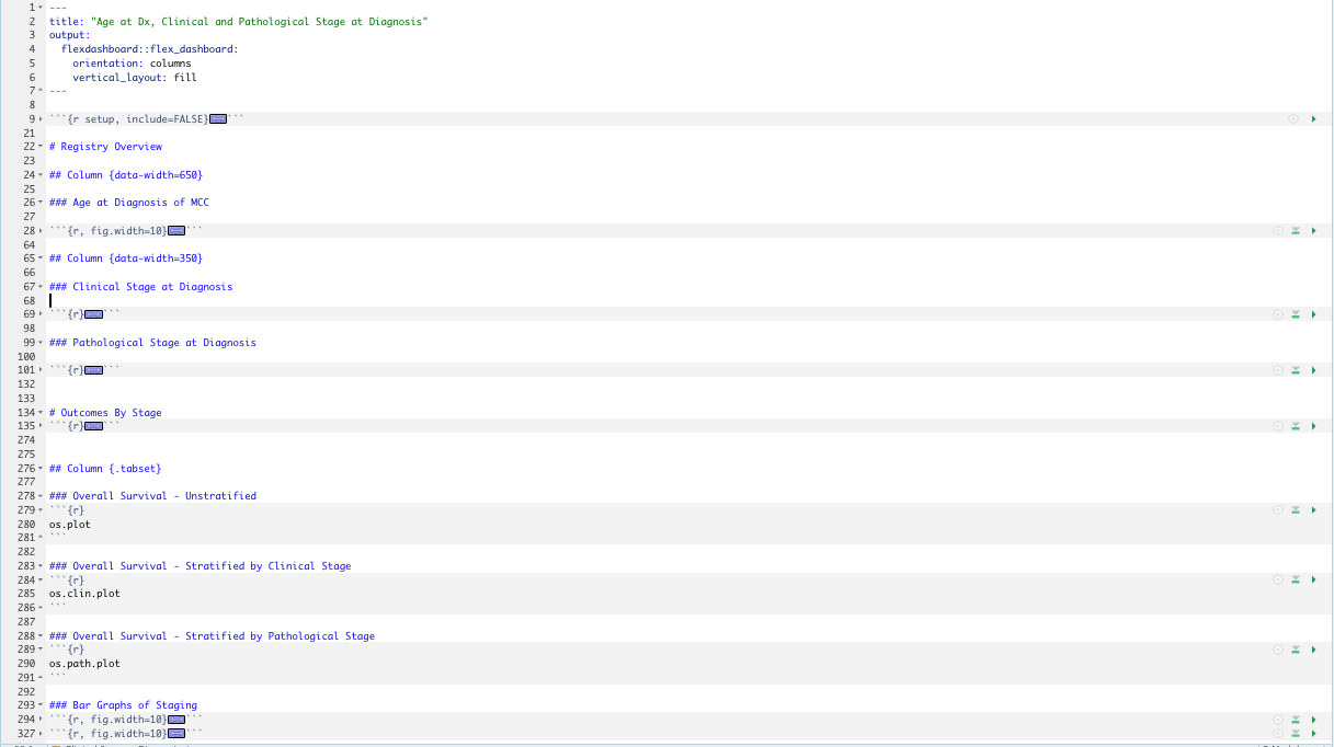
Additional FlexDashboard Formatting to Enhance the User Experience (UX)
Adding Pages to A FlexDashboard
- If you have numerous data visualizations in your dataset that you want to include in your FlexDashboard, dividing the dashboard into multiple pages can improve the overall UX
- Each page is defined by a level 1 markdown header, (#), and will have an individual navigation tab
- For example, in the data shown above, we may want to have the Age of Diagnosis of MCC boxplot on a page by itself, and the Clinical and Pathological Staging bar charts on a second page in the dashboard.
`# PAGE 1: Age at Diagnosis of MCC
### Chart A - Age at Diagnosis of MCC
dt <- read_excel("mcc_cohort_fake.xlsx") # Load the data
Age_at_Dx <- dt %>% select(record_id, age_at_dx) %>% drop_na(age_at_dx) # drop_na is a good function to eliminate rows that have missing values
Age_at_Dx$subjects <- "subjects" # add a column that unifies all the data (helpful for plotly)
Age_at_Dx %>% kable
plot_ly(data = Age_at_Dx, type = "box") %>%
  add_boxplot(x = Age_at_Dx$subjects, y = Age_at_Dx$age_at_dx,
              boxpoints = "all", jitter = 0.3, pointpos = -1.8,
              marker = list(color = 'rgb(7,40,89)'),
              line = list(color = 'rgb(7,40,89)'),
              color = I("steelblue4"),
              name = "MGH-HCC Cohort") %>%
  layout(title = "Age at Diagnosis of MCC")
`# PAGE 2: Staging of MCC
`## Column {data-width=350}
### Chart B - Clinical Stage at Diagnosis of MCC
cStage <-dt %>% select(record_id, man_clinstage, man_pathstage) %>% drop_na(man_clinstage) %>% filter(man_clinstage < 98)
cStageDF <- cStage %>% group_by(man_clinstage) %>% tally()
plot_ly(data = cStageDF) %>%
  add_bars(x = cStageDF$man_clinstage, y = cStageDF$n,
           color = I("steelblue4")) %>%
  layout(
    title = "Clinical Stage at Presentation",
    yaxis = list(title = "Number of Subjects"),
    xaxis = list(title = "Clincal Stage", ticktext = list("I", "IIA", "IIB", "III", "IV"), tickvals = list(0, 1, 2, 3, 4)))
### Chart C - Pathological Stage at Diagnosis of MCC
pStage <-dt %>% select(record_id, man_clinstage, man_pathstage) %>% drop_na(man_pathstage) %>% filter(man_pathstage < 6)
pStageDF <- pStage %>% group_by(man_pathstage) %>% tally()
plot_ly(data = pStageDF) %>%
  add_bars(x = pStageDF$man_pathstage, y = pStageDF$n,
           color = I("steelblue4")) %>%
  layout(
    title = "Pathological Stage at Presentation",
    yaxis = list(title = "Number of Subjects"),
    xaxis = list(title = "Pathological Stage", ticktext = list("I", "IIA", "IIB", "IIIA", "IIIB","IV"), tickvals = list(0, 1, 2, 3, 4, 5)))
This is what page 1 of the dashboard now looks like 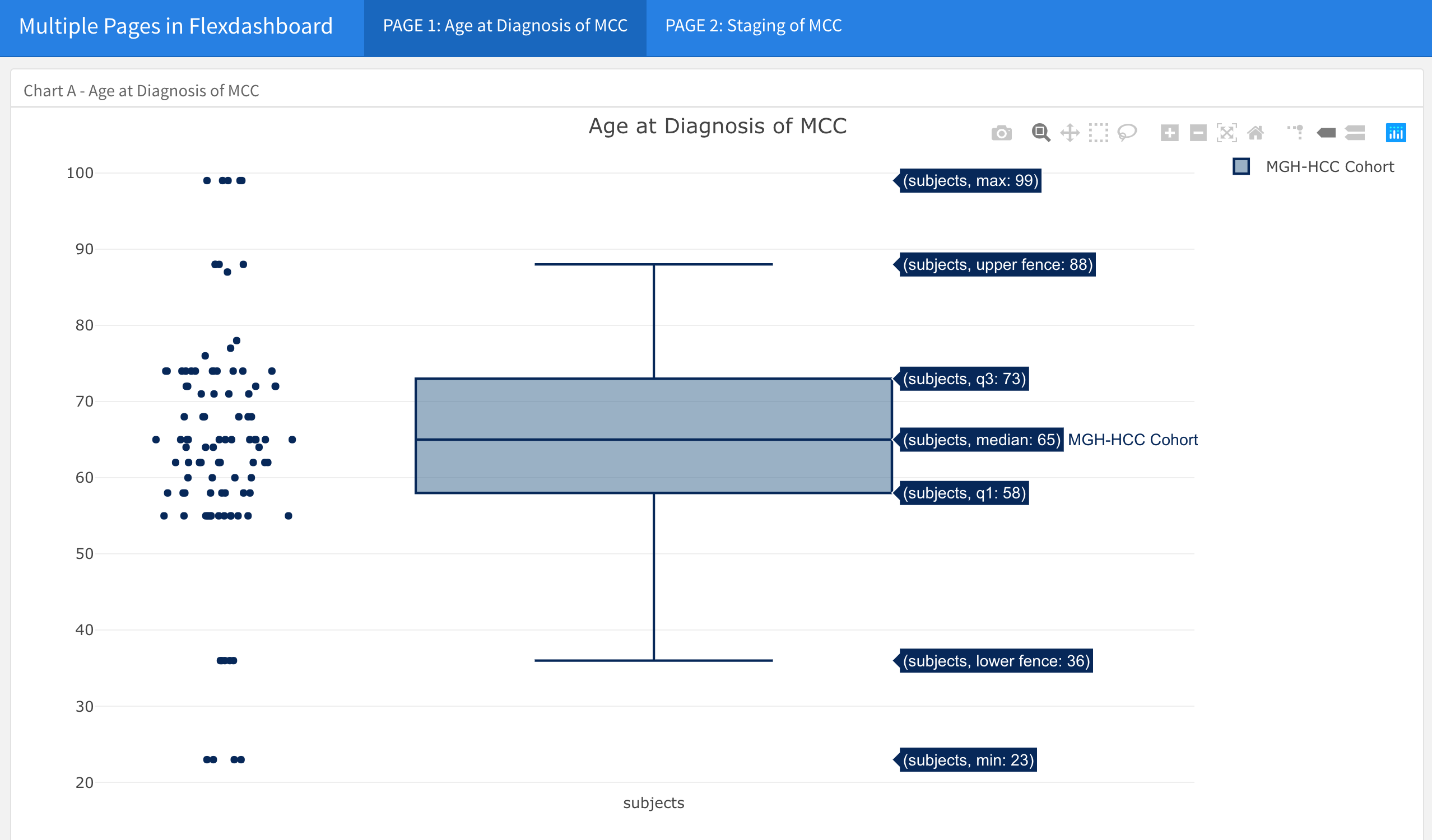
And this is what page 2 of the dashboard now looks like 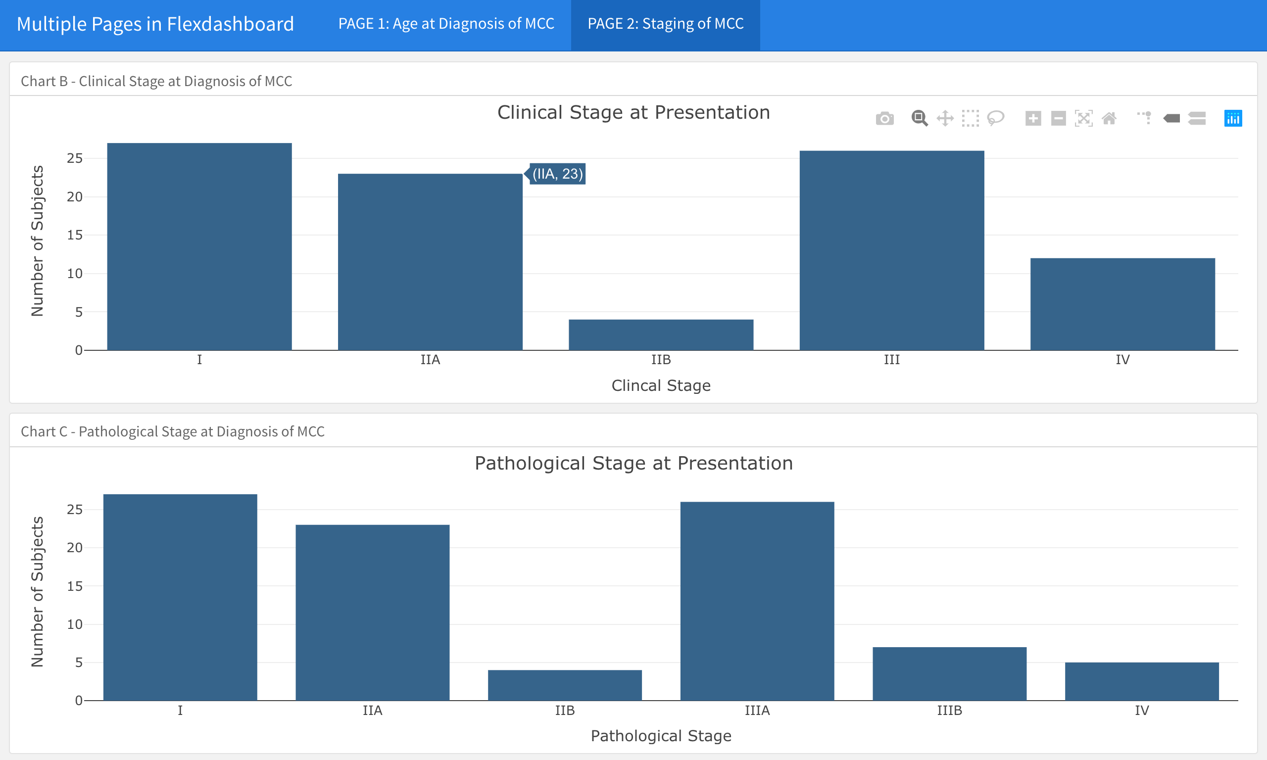
Add Tabs to A FlexDashboard
- If your Dashboard has a lot of content, you may also want to add tabs within pages to further layer the data presentation
- Instead of using
Column {data-width=350}above the dotted lines in your Flex DashBoard, useColumn {.tabset}
PAGE 1: Age at Diagnosis of MCC ======================================================
### Chart A - Age at Diagnosis of MCC
dt <- read_excel("mcc_cohort_fake.xlsx") # Load the data
Age_at_Dx <- dt %>% select(record_id, age_at_dx) %>% drop_na(age_at_dx) # drop_na is a good function to eliminate rows that have missing values
Age_at_Dx$subjects <- "subjects" # add a column that unifies all the data (helpful for plotly)
Age_at_Dx %>% kable
plot_ly(data = Age_at_Dx, type = "box") %>%
  add_boxplot(x = Age_at_Dx$subjects, y = Age_at_Dx$age_at_dx,
              boxpoints = "all", jitter = 0.3, pointpos = -1.8,
              marker = list(color = 'rgb(7,40,89)'),
              line = list(color = 'rgb(7,40,89)'),
              color = I("steelblue4"),
              name = "MGH-HCC Cohort") %>%
  layout(title = "Age at Diagnosis of MCC")
PAGE 2: Staging of MCC ======================================================
Column {.tabset}
- - - - - - - - - - - - - - - -
### Chart B - Clinical Stage at Diagnosis of MCC
cStage <-dt %>% select(record_id, man_clinstage, man_pathstage) %>% drop_na(man_clinstage) %>% filter(man_clinstage < 98)
cStageDF <- cStage %>% group_by(man_clinstage) %>% tally()
plot_ly(data = cStageDF) %>%
  add_bars(x = cStageDF$man_clinstage, y = cStageDF$n,
           color = I("steelblue4")) %>%
  layout(
    title = "Clinical Stage at Presentation",
    yaxis = list(title = "Number of Subjects"),
    xaxis = list(title = "Clincal Stage", ticktext = list("I", "IIA", "IIB", "III", "IV"), tickvals = list(0, 1, 2, 3, 4)))
### Chart C - Pathological Stage at Diagnosis of MCC
pStage <-dt %>% select(record_id, man_clinstage, man_pathstage) %>% drop_na(man_pathstage) %>% filter(man_pathstage < 6)
pStageDF <- pStage %>% group_by(man_pathstage) %>% tally()
plot_ly(data = pStageDF) %>%
  add_bars(x = pStageDF$man_pathstage, y = pStageDF$n,
           color = I("steelblue4")) %>%
  layout(
    title = "Pathological Stage at Presentation",
    yaxis = list(title = "Number of Subjects"),
    xaxis = list(title = "Pathological Stage", ticktext = list("I", "IIA", "IIB", "IIIA", "IIIB","IV"), tickvals = list(0, 1, 2, 3, 4, 5)))
This is the rmd of the FlexDashboard with the green arrow highlighting this critical line of code
![]()
This is now what page 2 of the dashboard looks like
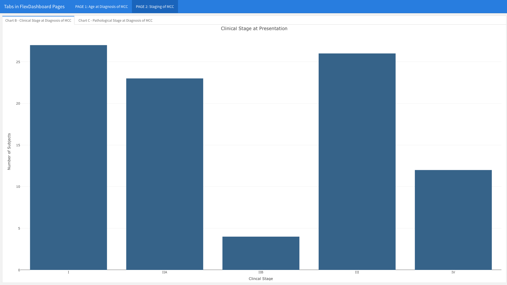
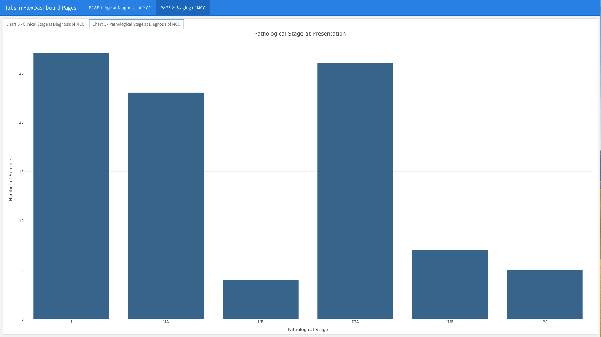
You will notice that the Clinical and Pathological Staging bar charts are no longer stacked in two rows on the same page. In contrast, you only see the Clinical Stage at Presentation graph, which takes up the entire page. You can see the tab in the upper left corner; if you click on the second tab, the chart for Pathological Stage at Presentation will emerge (see below).
Adding Side-by_Side Images Within a tabset Page
- If you want to have a section that has multiple tabset pages, for example as seen here
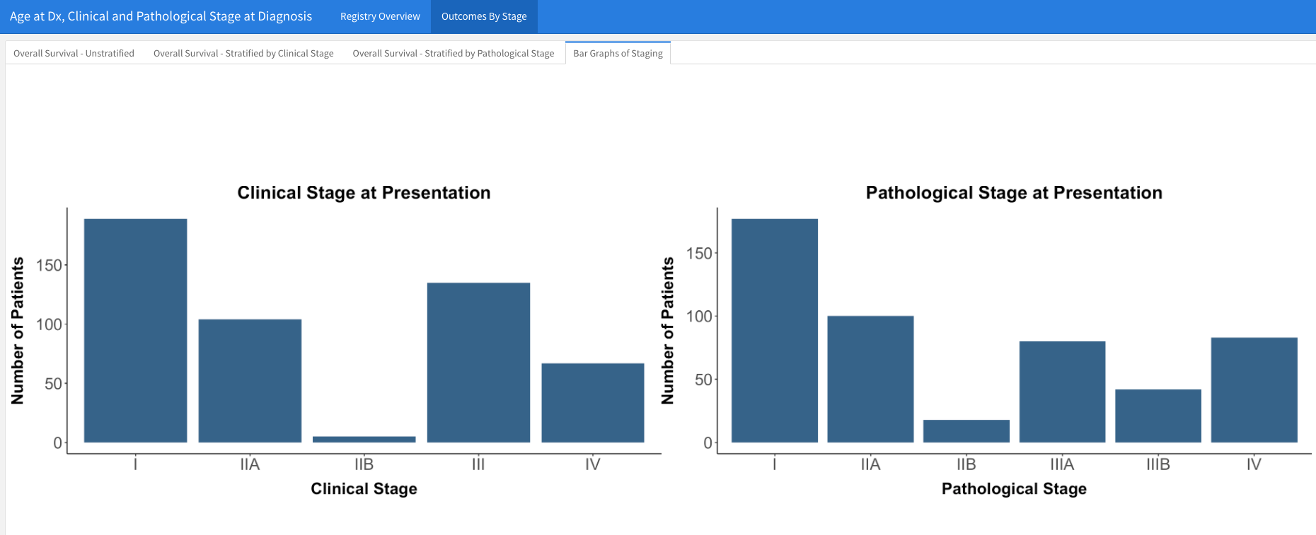
and then you want one of those pages to have side-by-side images (e.g.), you can use the following strategy
* Create the two graphs you would like side-by-side
* Save them both as objects
* Then within the level three header ### (as above Bar Graphs of Staging), use cowplot::plot.grid(image1, image2) to execute that graph
* For example, you can see the code we used here 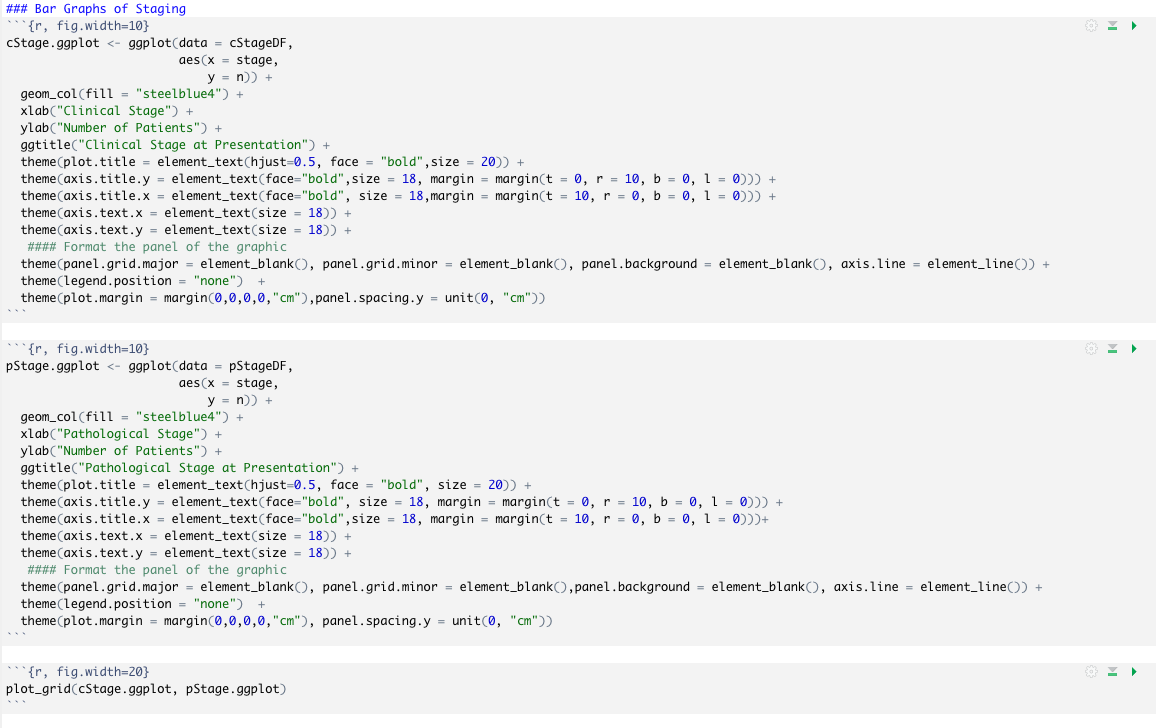
Take Home Points
- Dashboards are an excellent data visualization tool for Clinical and Translational Research
Flexdashboardis a great package to develop dashboards withR
- Adding pages and tabs to your dashboard can create a richer user experience for your intended audience
As always, please reach out to us with thoughts and feedback
Session Info
sessionInfo()R version 4.2.0 (2022-04-22)
Platform: x86_64-apple-darwin17.0 (64-bit)
Running under: macOS Big Sur/Monterey 10.16
Matrix products: default
BLAS: /Library/Frameworks/R.framework/Versions/4.2/Resources/lib/libRblas.0.dylib
LAPACK: /Library/Frameworks/R.framework/Versions/4.2/Resources/lib/libRlapack.dylib
locale:
[1] en_US.UTF-8/en_US.UTF-8/en_US.UTF-8/C/en_US.UTF-8/en_US.UTF-8
attached base packages:
[1] stats graphics grDevices utils datasets methods base
other attached packages:
[1] cowplot_1.1.1 scales_1.2.1 readxl_1.4.1
[4] plotly_4.10.1.9000 knitr_1.41 forcats_0.5.2
[7] stringr_1.5.0 dplyr_1.0.10 purrr_0.3.5
[10] readr_2.1.3 tidyr_1.2.1 tibble_3.1.8
[13] ggplot2_3.4.0 tidyverse_1.3.2 httr_1.4.4
[16] REDCapR_1.0.0 RCurl_1.98-1.7 flexdashboard_0.5.2
loaded via a namespace (and not attached):
[1] svglite_2.1.0 lubridate_1.9.0 assertthat_0.2.1
[4] digest_0.6.30 utf8_1.2.2 R6_2.5.1
[7] cellranger_1.1.0 backports_1.4.1 reprex_2.0.2
[10] evaluate_0.18 highr_0.9 pillar_1.8.1
[13] rlang_1.0.6 lazyeval_0.2.2 googlesheets4_1.0.1
[16] data.table_1.14.6 rstudioapi_0.14 rmarkdown_2.18
[19] webshot_0.5.3 googledrive_2.0.0 htmlwidgets_1.5.4
[22] munsell_0.5.0 broom_1.0.1 compiler_4.2.0
[25] modelr_0.1.10 xfun_0.35 systemfonts_1.0.4
[28] pkgconfig_2.0.3 htmltools_0.5.3 tidyselect_1.2.0
[31] viridisLite_0.4.1 fansi_1.0.3 crayon_1.5.2
[34] tzdb_0.3.0 dbplyr_2.2.1 withr_2.5.0
[37] bitops_1.0-7 grid_4.2.0 jsonlite_1.8.4
[40] gtable_0.3.1 lifecycle_1.0.3 DBI_1.1.3
[43] magrittr_2.0.3 cli_3.4.1 stringi_1.7.8
[46] fs_1.5.2 xml2_1.3.3 ellipsis_0.3.2
[49] generics_0.1.3 vctrs_0.5.1 kableExtra_1.3.4
[52] tools_4.2.0 glue_1.6.2 hms_1.1.2
[55] fastmap_1.1.0 yaml_2.3.6 timechange_0.1.1
[58] colorspace_2.0-3 gargle_1.2.1 rvest_1.0.3
[61] haven_2.5.1